Tariffs Without Truth: Turning the Industrial Policy Arms Race into a Rules-Based Truce
WTO paralysis spurs tariffs and subsidies—an industrial policy arms race
Replace blanket tariffs with evidence-based, sunset countervailing duties
Prioritize resilient skills; publish subsidy math to restore trust
 <
<
The Policy Illusion: Why Network Risk Still Rules Peripheral Economies
Interconnectedness keeps small, open economies exposed despite stronger policies
Dollar dominance—88% of FX trades, ~40% invoicing, $100T+ swaps—transmits shocks
Fix the plumbing: stress-test FX markets, add regional lines, tighten rules, expand local-currency invoicing

Why China’s Got a Problem with Stablecoins
China blocks stablecoins to guard monetary control
Goal: curb capital flight and AML risks; push users to e-CNY/mBridge
Ed-tech: use bank rails and e-CNY in China; stablecoins only abroad

Stop Chasing Androids: Why Real-World Robotics Needs Less Hype and More Science
Stop Chasing Androids: Why Real-World Robotics Needs Less Hype and More Science

Catherine McGuire is a Professor of Computer Science and AI Systems at the Gordon School of Business, part of the Swiss Institute of Artificial Intelligence (SIAI). She specializes in machine learning infrastructure and applied data engineering, with a focus on bridging research and large-scale deployment of AI tools in financial and policy contexts. Based in the United States (with summer/winter in Berlin and Zurich), she co-leads SIAI’s technical operations, overseeing the institute’s IT architecture and supporting its research-to-production pipeline for AI-driven finance.
Published
Modified
Humanoid robot limitations endure: touch, control, and power fail in the wild
Hype beats reality; only narrow, structured tasks work
Fund core research—tactile, compliant actuation, power—and use proven task robots

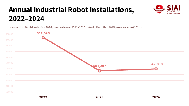
We don't have all-purpose robots because building them is more complicated than we thought. The world just keeps messing them up. Get this: about 4 million robots work in factories now—a record high!—but none of us see a humanoid robot fixing stuff around the house. Factory robots kill it with set tasks in controlled areas. Humanoids? Not so much when things get messy or unpredictable. That difference is a big clue. Sure, investors poured billions into humanoid startups in 2024 and 2025, and some companies were valued at insane levels. Reality check, though: dexterity, stamina, and safety are still big problems that haven't been solved. Instead of cool demos, we need to fund research into touch, control, and power. Otherwise, humanoids are stuck on stage.
Physics Is the First Problem for Humanoid Robots
Our bodies use about 700 muscles and receive constant feedback from sight, touch, and our own sense of position. Fancy humanoids brag about 27 degrees of freedom—which sounds cool for a machine, but it's nothing compared to us. It's not just about the number of parts. It's about how muscles and tendons stretch and adapt. And we sense way more than any robot. Even kids learn more, faster. A four-year-old has probably taken in 50 times more sensory info than those big language models, because they're constantly learning about the world hands-on. Simple: motors aren't muscles, and AI trained on text isn't the same as a body taught by the real world.
The limitations become evident when nuanced manipulation is required. Humanoid robots typically perform well on demonstration floors, but residential and workplace environments introduce variables. Friction may vary, lighting conditions can shift, and soft materials create obstacles. A robotic hand incapable of detecting subtle slips or vibrations will likely fail to retain objects. While simulation is beneficial, real-world deployment exposes compounding errors. Industry proponents acknowledge that current robots lack the sensorimotor skills that human experience imparts. Therefore, leading experts caution that functional, safe humanoids remain a long-term goal due to persistent physical challenges. Analytical rigor—not rhetoric—is necessary to address these realities.
The Economics Problem
Money doesn't solve everything. Figure AI got $675 million in early 2024 and was valued at $39 billion by September 2025. But cash alone won't turn a demo into a reliable worker. Amazon tested a humanoid named Digit to move empty boxes. That's something, but it proves that easy, single-purpose jobs in controlled areas are still the only wins right now. General-purpose work? Not there yet. It all depends on robots working reliably on different tasks. But so far, it's just limited tests.
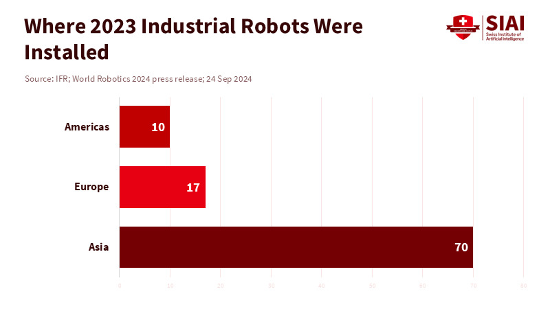
Then there's the energy issue. Work shifts are long, but batteries aren't. Agility says its new Digit lasts four hours on a charge, which is okay for set tasks with charging breaks. But that's not an eight-hour day in a messy place, let alone a home. Charging downtime, limited tasks, and a human babysitter make the business case weak. The robot market is growing, sure, but where conditions are perfect. Asia accounted for 70% of new industrial robot installations in 2023. But that doesn't mean humanoids are next; it just means tasks and environments need to be simple.
Quality counts too. Experts say that China's push for automation has led to breakdowns and durability issues, especially when parts are cheap. A recent analysis warned that power limits, parts shortages, and touch-sensitivity problems are blocking progress, even though marketing says otherwise. This doesn't mean there's no progress, but don't get carried away. Ignore this, and we'll waste money on demos instead of real research.
The Safety Problem
Safety isn't just a feeling. It's about standards. Factory robots follow ISO 10218, updated in 2025, which focuses on the whole job, not just the robot. Personal robots follow ISO 13482, which addresses risks and safety measures related to human contact. These aren't just rules. When a 60–70 kg machine with bad awareness falls over, it's dangerous, no matter how good the demo looks. Standards change slowly because people get hurt faster than laws can catch up.
That's why we should listen to the cautious voices. In late 2025, Rodney Brooks said we're over ten years from useful, minimally dexterous humanoids. Scientific American agrees: It's not just one missing part keeping humanoids out of our lives, but a lack of real-world smarts. If we make decisions based on flashy demos, we'll underfund research into touch, movement, and contact, where the real safety lies. The people who make standards will notice. We should too.
What to Fund: Research, Not Demos
The quickest way to address issues with humanoid robots is to improve their movement. Human muscles adjust to stiffness and give way a little. Electric motors don't. We need variable-impedance systems, tendon-driven designs, and soft robots that give way on contact. The goal isn't cool moves, but coping with the messy world. Tie funding to damage reduction, not cheering. If a hand can open a jar without smashing it—or know when to give up—that's worth paying for.
Next is touch. High-resolution touch sensors will change the way robots grab, more than hours of watching YouTube videos. We need lots of varied touch data, like a kid learning by making a mess. As LeCun says, without more data, robot smarts will stall. The answer is on-device data collection in living labs that look like kitchens and classrooms—with simulators that get friction right. Otherwise, the real world will always be out of reach.
Lastly, we need stamina. Warehouse work is long; homes are messy. Up to four hours of battery life is a start, but it limits what robots can do. Improving energy density is slow. And safety around heat and charging is vital. We need research into battery design, safe, fast charging, and graceful ways to shut down when power drops. And we need rules that punish duty-cycle claims that don't hold up. We should measure time between breakdowns, not marketing hype.
What should schools do?
Stop selling students on Android fantasies. Teach controls, sensing, safety, and testing. These skills apply to mobile robots, surgery systems, and factory automation, where the jobs are. Second, build industry labs where students test products on real materials and in messy conditions, with safety experts on hand. Third, reward designs that fail safely and recover, not just ones that work once. We need engineers who can turn cool demos into working systems.
Admins should use robots only for clear, low-risk tasks. Assign humanoids to simple workflows, as Amazon does, where mistakes are easy to fix. Invest the rest in other proven automation—like AMRs, fixed arms, and inspection systems. Use complex data—uptime, breakdowns, accidents—to guide decisions. Halt projects that don’t lead to reliable production. Politicians should back robotics projects with open results, not just hype. Ensure funding and incentives are tied to reporting failures, safety audits, and real-world testing. Support the development of sensors, actuators, and power systems that benefit many users. Advocate strict safety limits for heavy robots until risks are proven manageable.
Here's the practical test: The next three years, if we can build a robot that can fold T-shirts, carry a pot without spilling, and recover from a fall without help, we're onto something. These tasks aren't fun, but they touch on the physics, sensing, and control needed to deal with the real world. Solve them, and a safer service is possible. Skip them, and the hype will keep going, louder but not smarter. Let's be real. Investors will keep hyping. Press releases will hype robots. Some tests will work. But the robot future is still focused on machines doing specific jobs in specific places. That's valuable. It boosts productivity in boring places that pay the bills. The all-purpose humanoid will appear only when we earn it, by funding the unglamorous science of contact, control, and power.
Millions of robots are now in use, but almost none are humanoids in public. That's not a lack of imagination; it's reality. In robotics, the action is where limits can be designed and tested. The hype is somewhere else. If we want safe androids someday, we must change the system. Support touch sensors that last, actuators that give way, and batteries that work without trouble. Demand real tests, not just videos. Treat humanoid issues as research, not branding. Do this, and we might see a robot we can trust on the sidewalk.
The views expressed in this article are those of the author(s) and do not necessarily reflect the official position of the Swiss Institute of Artificial Intelligence (SIAI) or its affiliates.
References
Agility Robotics. “Agility Robotics Announces New Innovations for Market-Leading Humanoid Robot Digit.” March 31, 2025.
Amazon. “Amazon announces 2 new ways it’s using robots to assist employees and deliver for customers.” Company news page.
International Federation of Robotics (IFR). “Industrial Robots—Executive Summary (2024).”
International Federation of Robotics (IFR). “Record of 4 Million Robots in Factories Worldwide.” Press release.
Innerbody. “Interactive Guide to the Muscular System.”
Reuters. “Robotics startup Figure raises $675 mln from Microsoft, Nvidia, other big techs.” Feb. 29, 2024.
Reuters. “Robotics startup Figure valued at $39 billion in latest funding round.” Sept. 16, 2025.
Rodney Brooks. “Why Today’s Humanoids Won’t Learn Dexterity.” Sept. 26, 2025.
Scientific American. “Why Humanoid Robots Still Can’t Survive in the Real World.” Dec. 13, 2025.
The Economy (economy.ac). “China tops 2 million industrial robots, but quality concerns persist.” Nov. 2025.
The Economy (economy.ac). “Humanoid Robots and the Division of Labor: bottlenecks persist.” Nov. 2025.
TÜV Rheinland. “ISO 10218-1/2:2025—New Benchmarks for Safety in Robotics.”
Unitree Robotics. “Unitree H1—Full-size universal humanoid robot (specifications).”
Yann LeCun (LinkedIn). “In 4 years, a child has seen 50× more data than the biggest LLMs.”
Catherine McGuire is a Professor of Computer Science and AI Systems at the Gordon School of Business, part of the Swiss Institute of Artificial Intelligence (SIAI). She specializes in machine learning infrastructure and applied data engineering, with a focus on bridging research and large-scale deployment of AI tools in financial and policy contexts. Based in the United States (with summer/winter in Berlin and Zurich), she co-leads SIAI’s technical operations, overseeing the institute’s IT architecture and supporting its research-to-production pipeline for AI-driven finance.


China's iron ore strategy has become a key battleground in the U.S.-China resource conflict
China centralizes iron ore power
Simandou adds leverage and options
Train procurement to protect budgets

In late 2025, China, which accounts for almost three-quarters of the world's seaborne iron
Paying Good Teachers More – The Key to Better Education
Raise base pay to close gaps and stabilize schools
Use low-bias bonuses to retain high-impact teachers in hard posts
Pair pay reform with clean screening and clear metrics to lift quality

We’re facing a serious problem:
Insider Trading by Politicians Is About Power, Not Secrets
Leadership brings the trading edge; power beats tips
Buys precede contracts, sales precede heat—disclosure failed
Ban lawmakers’ individual stocks or require true blind trusts

Here's the t
Take It Down, Keep Moving: How to Take Down Deepfake Images Without Stalling U.S. AI Leadership
Take It Down, Keep Moving: How to Take Down Deepfake Images Without Stalling U.S. AI Leadership

Ethan McGowan is a Professor of AI/Finance and Legal Analytics at the Gordon School of Business, SIAI. Originally from the United Kingdom, he works at the frontier of AI applications in financial regulation and institutional strategy, advising on governance and legal frameworks for next-generation investment vehicles. McGowan plays a key role in SIAI’s expansion into global finance hubs, including oversight of the institute’s initiatives in the Middle East and its emerging hedge fund operations.
Published
Modified
48-hour takedowns for non-consensual deepfakes
Narrow guardrails curb abuse, not innovation
Schools/platforms: simple, fast reporting workflows

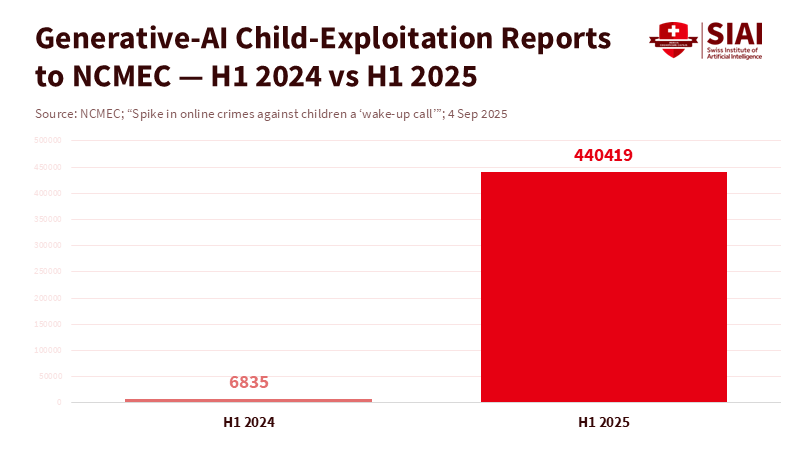
Deepfake abuse is a vast and growing problem. In the first half of 2025, the U.S. CyberTipline received 440,419 reports alleging that generative AI was used to exploit kids. That's a 64 times increase from 2024! This causes harm every single day, so we really need to put some protections in place, and fast. The Take It Down Act aims to quickly remove deepfake images without disrupting America's AI progress. Some people worry that rules might slow things down and let China get ahead. But we need to make sure tech improves while keeping people safe. The Act shows we can protect victims and encourage AI leadership at the same time.
What the Act Does to Get Rid of Deepfake Images
This law is all about what works. It makes it illegal to share private images online without permission, including real photos and AI-generated ones. Covered platforms have to create a simple system for people to report these images so they can be taken down. If a victim sends a genuine request, the platform must delete the content within 2 days and do its best to remove any copies it knows about. The Federal Trade Commission can punish those who aren't following the rules. The penalties are harsher if minors are involved, and it's illegal to threaten to publish these images, too. It's all about promptly removing deepfake images once a victim speaks up. Platforms have until May 19, 2026, to get this system up and running, but the criminal stuff is already in place.
The details matter. Covered platforms are websites and apps that are open to the public and primarily host user-generated content. Internet providers and email are omitted. The Act has a good-faith clause, so platforms that quickly remove stuff based on clear evidence won't get in trouble for taking down too much. It doesn't replace any state laws, but it adds basic protection at the federal level. Basically, Congress is bringing the straightforward approach of copyright takedowns to a situation where delays can cause significant problems, especially for children. This law is targeting things that can't be defended as free speech. It's about non-consensual, sexual images that cause real harm. That's why, unlike many other AI proposals in Washington, this one became law.
What the Law Can and Can't Do to Remove Deepfake Images
The Act is a response to a significant increase in AI being used for exploitation. Getting stuff taken down fast is super important because a single file can spread quickly across the internet. The two-day rule helps prevent lasting damage. The urgency of the Act shows just how much harm delayed removal causes victims.
But a law that focuses on what we can see might miss what's going on behind the scenes. Sexual deepfakes grab headlines. Discriminatory algorithm decisions often don't. If you get turned down for credit, housing, or a job by an automated system, you might not even know a computer made that decision or why. Recent studies suggest that lawmakers should take these less-obvious AI harms just as seriously as the more visible ones. They suggest things like impact assessments, documentation, and solutions that have as much power as what this Act gives to deepfake victims. If we don't have these tools, the rules favor what shocks us most over what quietly limits opportunity. We should aim for equal protection: quickly remove deepfake images and be able to spot and fix algorithmic bias in real time.
There's also a limit to how many takedowns can do. The open internet can easily get around them. The most well-known non-consensual deepfake sites have shut down or moved under pressure, but the content ends up on less-obvious sites and in private channels, and copies pop up all the time. That's why the Act says platforms need to remove known copies, not just the original link. Schools and businesses need ways to go from the first report to platform action to getting law enforcement involved when kids are involved. The Act gives victims a process at the federal level, but these place needs a system to support it.
Innovation, Competition, and the U.S.–China Dynamic
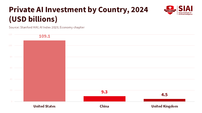
Will this takedown rule slow down American innovation? The stats say no. In 2024, private AI investment in the U.S. hit \$109.1 billion, almost twelve times China's \$9.3 billion! The U.S. is also ahead in creating important models and funding AI projects. A clear rule about non-consensual private images won't undermine those numbers. Good rules actually reduce risks for place that need to use AI while following strict legal and ethics guidelines. Safety measures aren't bad for innovation; they encourage responsible use.
A lot is happening with laws in the U.S. Right now. In 2025, states were considering many AI-related bills. A lot of them mentioned deepfakes, and some became law. Many are specific to certain situations, some don't agree with each other, and a few go too far. This could be a problem if it leads to changing targets. The government has suggested one-rulebook ideas to limit what states can do, but businesses disagree on if that would help. What we should be doing is improving coordination. Keep the Take It Down rules as a foundation, while adding requirements based on risks. Stop state measures only when they really cause conflicts. Focus on promoting what's clear, not what's confusing.
What Schools and Platforms Should Do Now to Remove Deepfake Images
Schools can start by sharing a simple guide that tells people how to report incidents and includes legal information in digital citizenship programs. Speed and guidance are key, connecting victims to counseling and law enforcement when needed.
Platforms should use the next few months to test things out. Pretend to receive a report, check it, remove the file, search for and delete identical copies, and document everything. Take the takedown process to all areas where content spreads, like the web, mobile, and apps. If your platform allows third-party uploads, make sure one victim report reaches every location where the host assigns an internal ID. Platforms should release brief reports on response times as we get closer to May 19, 2026. The extra hour you save now could prevent problems later. For smaller platforms, following the pattern from DMCA workflows can lower risks and engineering costs.
Beyond Takedown: Building More Trust
The Act gives us a chance. Use it to raise the standards. First, invest in image authentication where it is most important. Schools that use AI should use tools that support tracking image origin. This won’t spot everything, but it will link doubts to data. Second, make sure people can see when an automated tool was used and challenge it where it is essential. This is like what the Act grants to deepfake victims: a way to say, That's wrong, fix it”. Third, treat trust work as a means of growth. America doesn't fall behind by making places safer. It gains adoption and lowers risks while keeping the pipeline of students and nurses open.
The amount of deepfakes will increase. That shouldn’t stop research. People should ensure that clear notice forms are in place and uphold a duty of care for kids. The Act does not solve every AI problem. But by prioritizing response & transparency, we can build trust in AI’s potential. Take steps now to show your commitment to innovation.
We started with a scary issue. This underlines the need for action. The Take It Down Act requires platforms to remove content. The law is clear. It won't fix it, others will need to be addressed. It will not end the battle between creators & censors. But it will allow control & and we can remove deepfake images. This is we should seek: a cycle of trust
The views expressed in this article are those of the author(s) and do not necessarily reflect the official position of the Swiss Institute of Artificial Intelligence (SIAI) or its affiliates.
References
Brookings Institution. (2025, December 11). Addressing overlooked AI harms beyond the TAKE IT DOWN Act.
Congress.gov. (2025, May 19). S.146 — TAKE IT DOWN Act. Public Law 119-12. Statute at Large 139 Stat. 55 (05/19/2025).
MultiState. (2025, August 8). Which AI bills were signed into law in 2025?
National Center for Missing & Exploited Children. (2025, September 4). Spike in online crimes against children a “wake-up call”.
National Conference of State Legislatures. (2025). Artificial Intelligence 2025 Legislation.
Skadden, Arps, Slate, Meagher & Flom LLP. (2025, June 10). ‘Take It Down Act’ requires online platforms to remove unauthorized intimate images and deepfakes when notified.
Stanford Human-Centered AI (HAI). (2025). The 2025 AI Index Report (Key Findings).
Ethan McGowan is a Professor of AI/Finance and Legal Analytics at the Gordon School of Business, SIAI. Originally from the United Kingdom, he works at the frontier of AI applications in financial regulation and institutional strategy, advising on governance and legal frameworks for next-generation investment vehicles. McGowan plays a key role in SIAI’s expansion into global finance hubs, including oversight of the institute’s initiatives in the Middle East and its emerging hedge fund operations.
The Missing Middle of Teen Chatbot Safety
The Missing Middle of Teen Chatbot Safety
Ethan McGowan is a Professor of AI/Finance and Legal Analytics at the Gordon School of Business, SIAI. Originally from the United Kingdom, he works at the frontier of AI applications in financial regulation and institutional strategy, advising on governance and legal frameworks for next-generation investment vehicles. McGowan plays a key role in SIAI’s expansion into global finance hubs, including oversight of the institute’s initiatives in the Middle East and its emerging hedge fund operations.
Published
Modified
Teen chatbot safety is a public-health issue as most teens use AI daily
Adopt layered age assurance, parental controls, and a school “teen mode” with crisis routing
Set a regulatory floor and publish safety metrics so safe use becomes the default

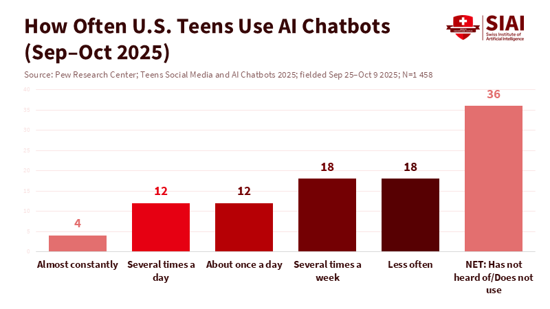
Here’s a stat that should grab your attention: around 64% of U.S. teens are using AI chatbots now, and about a third use them every day. So, teen chatbot safety isn’t a small thing anymore; it’s just part of their daily online lives. When something becomes a habit, little slip-ups can turn into big problems: like bad info about self-harm, wrong facts about health, or a late-night so-called friend that messes up ideas about consent.
The real question isn’t if teens are using chatbots—they clearly are—but if schools, families, and the platforms themselves can come up with rules that keep up with how fast and intensely these tools are being used. We need to switch from just letting anyone jump in with no rules to having a more protective approach focused on stopping problems before they start. We can’t just say it’s good enough for adults. It needs to be safe enough for kids. That bar needs to be higher, and it should’ve been raised already.
Why Teen Chatbot Safety is a Health Concern
Teens aren’t just using these things for homework anymore; they’re using them for emotional support. In the UK, the numbers show that one in four teens asked AI for help with their mental health in the last year, usually because getting help from real people felt slow, judgmental, or harsh. A U.S. survey shows most teens have messed around with chatbots, and a bunch use them daily. This combo of using them a lot and having secret chats makes things risky when the chatbot answers wrong, isn’t clear, or acts too sure of itself. It also makes it seem normal to have a friend who’s always there. This isn’t harmless; it changes how teens think about advice, being on their own, and asking for help.
If something has so much influence, then it needs safety measures built in. The proof is there now: teens are using chatbots a lot and for serious stuff. Policies have to treat this as ongoing, not just as an app you download once. A serious event prompted people to demand action. In September 2025, a family said their teen’s suicide came after months of talking to a chatbot. After that, OpenAI said it would check ages and give answers made for younger users, mainly dealing with thoughts of suicide. This came after earlier talk about maybe telling the authorities if there were signs of self-harm. That was a touchy subject, but it showed that this whole thing has risks.Heavy, unsupervised use when you’re young and unsure—that’s what makes persuasive but sometimes wrong systems risky. If the main user is a kid, then the people in charge need to do what they can to keep them away from stuff that could hurt them.
From Asking Your Age to Actually Knowing It: Making Teen Chatbot Safety Work
There are some basic rules already. Big companies make you be at least 13 to use their stuff, and if you’re under 18, you need a parent’s okay. In 2025, OpenAI introduced parental controls so parents and teens could link accounts, set limits, block features, and add extra safety. The company also discussed using a system to guess your age and check IDs so users get the correct settings and less risky content. These are must-haves; they’re better than just asking people to tell on themselves. Of course, getting consent has to mean something. Controls have to be on point and tough to get around. Mainly, protecting kids should be the priority, especially at night when risky chats tend to happen.
Knowing a user’s age should be a system, not just a one-time thing. Schools and families need different layers of protection, including account settings, device rules, and safety features for younger users. Policies should ensure you’re checking for risks in a real way, including spotting potential failures (for example, incorrect information), putting controls in place, measuring how things are going, and making changes when needed.
In other words, safety for teens on chatbots should mean stricter rules for touchy subjects, set times when they can’t be used, blocking lovey-dovey or sexual stuff, and making it easy to get help from a real person if there’s a serious problem—all while keeping their info private and not causing unnecessary alarms. The standard should be pretty darn sure, and you should have to prove it. All these rules are key to making sure promises turn into real action.
A Schools First Idea for Teen Chatbot Safety
Schools are right in the middle of all this, but policies often treat them like they don’t matter. Surveys from 2024 and 2025 found that many teens are using AI to help with schoolwork, often without teachers even knowing. A lot of parents think schools haven’t said much about what’s okay and what’s not. We can fix this gap. School districts can put a simple, doable plan in place: have different levels of access based on what you’re doing, have people check things over, and have clear rules about data.
What I mean is, there should be one mode for checking facts and writing stuff with sources, and another, more strict mode for deep or emotional questions. A teacher should be able to see what the student is doing, what they’re asking about, and a short reason why it’s okay on their device. Data rules need to be clear: don’t train the AI using student chats, keep logging to a minimum, and have set rules for deleting data. Schools are already doing this for search engines and videos, so they should do it for chatbots too.
School safety for teen chatbots should also include social skills, not just tech barriers. Health teachers should show how to find proof and spot wrong answers. Counselors should deal with risks flagged by the tools. School leaders should set rules about using them at night related to going to class and feeling okay. Companion chatbots need extra thought. Studies show that teens can become emotionally attached to fake friends, which can blur boundaries and lead to advice that encourages controlling behavior. Schools can ban romantic companions on devices they control while still allowing educational tools, explaining why: consent, feeling for others, and real-world skills don’t come from being alone. It’s not about scaring kids; it’s about guiding them toward learning and keeping them away from the parts of adolescence that are easiest to mess with.
Thinking About the Criticisms—and How to Answer Them
Criticism one: Checking ages might invade privacy and mislead users. That’s true, so the best designs should start with predicting ages using the device, use rules that can be adjusted, and only check IDs when there’s a serious risk, and you have permission. There are clear guides on making sure the methods fit the risk: reduce risks using the least intrusive ways that still get the job done, keep track of mistakes, and write down the trade-offs. Schools can further reduce risk by ensuring the checks aren’t part of a student’s school record and by not saving raw images when estimating faces. Telling everyone what’s going on is key: share the error rates, tell teens and parents how they can argue a decision, and allow people to report misuse secretly. If we do these things, teen chatbot safety can move forward without turning every laptop into a spy tool.
Criticism two: Strict safety measures might make inequality even worse, since students with their own devices might get around the school rules and end up doing better. The answer is to create safe access, the easiest way to do things everywhere. Link school accounts to home devices using settings that move with them, apply the same modes and quiet hours across the board, and don’t train the AI on student data so families can trust the tools. When the simplest thing is also the safest, fewer students will try to cheat the system.
And the idea that safety measures stop learning just ignores what’s happening now: teens are already using chatbots for quick answers. A better design can raise the bar by asking for sources, showing different points of view, and controlling the tone when dealing with touchy subjects involving kids. Everyone does better when every student has access in a set way, rather than when some people can buy their way around the safety measures.
What the People in Charge Should Do Next
To policymakers, that reads: Do it now—make sure any chatbot teens use meets these three rules. First, make age checks real: start with the least nosey way possible, and only go further as needed. Also, have independent audits to find any biases and mistakes. Second, make sure there’s a teen mode that blocks certain features, uses a calmer tone for emotional times, strictly blocks sexual stuff and companions, and makes it easy to get help from a real person in an emergency. Third, demand tools that are ready for schools: admin controls, limited access based on the task, minimal data, and a public safety card that outlines the protections for teens.
These protections ensure older teens can access more advanced content with permission, while still guaranteeing the tools fit what teens need. Refer to risk management guides in all rules so agencies know how to monitor for compliance. Do it now to protect teens in their online lives.
Platforms should share their youth safety numbers regularly. How often do the teen-mode models block stuff they shouldn’t? How usually do crises come up, and how fast do real people jump in? What’s the rate of getting ages wrong? What are the top three areas where teens are getting wrong info, and what fixes have been made? Without these numbers, safety is just a way to sell something. If we share these numbers, safety becomes real. Independent researchers and youth safety groups should be part of the process.
Current work from people who study cyberbullying shows the new risks of companion interactions and sets a plan for schools to research this. Policymakers can provide funding to connect school districts, researchers, and companies to test teen modes in the real world and compare outcomes across different safety plans. The standard should be something everyone can see, not just something some company owns: Teen chatbot safety gets better when problems are out in the open.
The truth is, chatbots are now part of the daily lives of millions of teens. That’s not going to change. The only choice we have is whether we create systems that admit teens are using these things and do a good job of dealing with that. We already have everything we need: age checks that are better than just clicking a box, parental controls that actually link accounts, school systems that block risky stuff while pushing good habits, and audits to make sure the guardrails are doing their job. This isn’t about attacking technology. It’s just about being responsible and making sure things are safe in a world where advice can come instantly and sound super sure. Set the bar. Measure what matters. Share what you find. If we do all this, teen chatbot safety can move from being just a catchy phrase to being something real. And the odds of seeing news stories about problems we could have stopped will go way down.
The views expressed in this article are those of the author(s) and do not necessarily reflect the official position of the Swiss Institute of Artificial Intelligence (SIAI) or its affiliates.
References
Common Sense Media. (2024, June 3). Teen and Young Adult Perspectives on Generative AI: Patterns of Use, Excitements, and Concerns.
Common Sense Media. (2024, September 18). New report shows students are embracing artificial intelligence despite lack of parent awareness and…
Common Sense Media. (2024). The Dawn of the AI Era: Teens, Parents, and the Adoption of Generative AI at Home and School.
Cyberbullying Research Center. (2024, March 13). Teens and AI: Virtual Girlfriend and Virtual Boyfriend Bots.
Cyberbullying Research Center. (2025, January 14). How Platforms Should Build AI Chatbots to Prioritize Youth Safety.
NIST. (2024). AI Risk Management Framework and Generative AI Profile. U.S. Department of Commerce.
OpenAI. (2024, Dec. 11). Terms of Use (RoW). “Minimum age: 13; under 18 requires parental permission.”
OpenAI. (2024, Oct. 23). Terms of Use (EU). “Minimum age: 13; under 18 requires parental permission.”
OpenAI. (2025, Sep. 29). Introducing parental controls.
OpenAI Help. Is ChatGPT safe for all ages? “Not for under-13; 13–17 need parental consent.”
Pew Research Center. (2025, Dec. 9). Teens, Social Media and AI Chatbots 2025.
Scientific American. (2025). Teen AI Chatbot Usage Sparks Mental Health and Regulation Concerns.
The Guardian. (2025, Sep. 11). ChatGPT may start alerting authorities about youngsters considering suicide, says Altman.
The Guardian. (2025, Sep. 17). ChatGPT developing age-verification system to identify under-18 users after teen death.
TechRadar. (2025, Sep. 2 & Sep. 29). ChatGPT parental controls—what they do and how to set them up.
Ethan McGowan is a Professor of AI/Finance and Legal Analytics at the Gordon School of Business, SIAI. Originally from the United Kingdom, he works at the frontier of AI applications in financial regulation and institutional strategy, advising on governance and legal frameworks for next-generation investment vehicles. McGowan plays a key role in SIAI’s expansion into global finance hubs, including oversight of the institute’s initiatives in the Middle East and its emerging hedge fund operations.
Italy’s Fiscal Rehab, France’s Drift, and Why US Fiscal Sustainability Now Shapes Education
US fiscal sustainability is strained; interest now tops defense
Italy rebounds with primary surpluses; France lags with 5%+ deficits
A near-term US primary surplus would stabilize debt and shield education