Chinese subsidies have tilted global markets in favor of state-backed firms
WTO rules have failed to keep pace with this shift
Fair trade now depends on coordinated reform and enforcement
Integrating Physical AI Platforms into Education: A Forward-Thinking Policy Approach
Picture
Member for
1 year 8 months
Real name
Catherine McGuire
Bio
Professor of AI/Tech, Gordon School of Business, Swiss Institute of Artificial Intelligence
Catherine McGuire is a Professor of Computer Science and AI Systems at the Gordon School of Business, part of the Swiss Institute of Artificial Intelligence (SIAI). She specializes in machine learning infrastructure and applied data engineering, with a focus on bridging research and large-scale deployment of AI tools in financial and policy contexts. Based in the United States (with summer/winter in Berlin and Zurich), she co-leads SIAI’s technical operations, overseeing the institute’s IT architecture and supporting its research-to-production pipeline for AI-driven finance.
Published
Modified
Physical AI moves intelligence from screens into systems that act in the real world
In education, AI shifts from a tool to shared infrastructure with new governance risks
The policy challenge is managing embodied intelligence at institutional scale
Automation is changing the world quickly. For example, factories added 4.28 million robots by 2023, a 10% increase in just one year. Now, intelligence is moving from distant data centers into machines that interact directly with the physical world. This shift means education policy must adapt quickly, as integrated systems combining software, sensors, processing, and mechanical components are becoming the norm. The main challenge is ensuring schools understand and address the mix of hardware, local processing, safety, and workforce changes as AI becomes both a physical and a digital force.
As AI moves from digital tools to physical devices, schools need a new way to bring technology into classrooms.
We need to change our approach. In the past, most discussions of AI in schools focused on software applications, such as content moderation, plagiarism detection, and personalized learning. These are still important, but now we should see software, hardware, and mechanical parts as components of a single system. This matters because spending, risks, and opportunities now overlap in the buying and use of these tools. When a school district buys an adaptive learning program, it’s not just a software license—they also deal with data sent to the cloud, on-site hardware, warranties, and safety steps for devices that can move, talk, or sense their surroundings. These changes affect budgets, teacher training, and fairness. Hardware depreciates differently from software, so maintenance costs are important but often overlooked. If schools treat these areas separately, they may misjudge costs and risks.
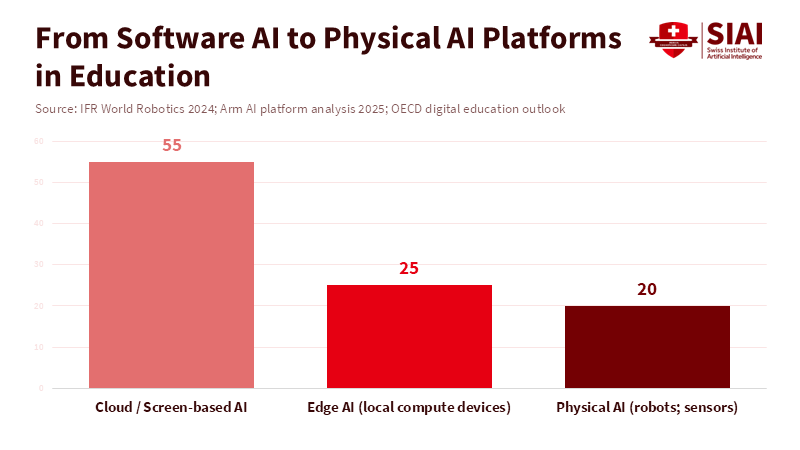
Figure 1: AI in education is no longer concentrated in the cloud; physical and edge systems now represent a growing share of deployed intelligence.
The numbers show strong growth. In 2023, there were about 4.28 million industrial robots in use, with more than half a million new ones added each year. This shows that physical systems are becoming common in many industries. The market for local AI processing is also growing fast and could reach tens of billions of dollars by 2024 or 2025. Venture funding for robotics and hardware-based AI has bounced back from 2022–2023, now reaching billions of dollars each year, mostly going to startups that blend on-device analytics with autonomous features.
Implications for Learning Environments and Curriculum Development
Moving to physical AI platforms changes what schools need to teach and maintain. Hardware skills are now essential. Teachers will need to manage devices that interact with students and classrooms, such as voice-activated tools, delivery robots, and environmental sensors. Buying teams must check warranties, update policies, and handle vendor relationships. Facilities staff should plan for charging stations, storage, and safety areas. Special education teams need to update support plans for new robotic tools that help with movement or sensory needs. Costs also need a fresh look. While software can be used by many, hardware incurs upfront costs, depreciates over time, and requires regular upkeep. Over five years, the total cost of classroom devices could exceed that of software if schools don’t plan for group purchases, shared services, or local repair centers.
AI devices can take over repetitive or routine tasks, letting teachers focus on students and advanced topics. Virtual assistants help with scheduling, grading, and paperwork. However, these benefits require reliable support and maintenance, or pilot programs risk failing. Policies should connect device funding to technical training and regular performance reviews.
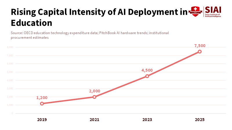
Figure 2: As AI becomes physical, education systems face hardware-style cost curves rather than software-style scaling.
Governance, Safety, and Workforce Policies for Physical AI Platforms
Bringing physical AI into schools creates new challenges for rules and oversight. Physical systems can fail in different ways, such as sensor errors, mechanical breakdowns, or poor decisions. Rules designed for software problems are not enough for robots capable of causing real-world harm. Regulators need to set up standard safety checks that test software, stress-test hardware, and look at how people use the systems. These checks should compare different systems directly. For privacy, processing data on-site means less student data goes to the cloud, but it also brings up concerns about data logs, device software, and data sent to vendors. Policies should limit what is recorded on devices, clarify data handling, and require regular external audits.
Policymakers also need to focus on workforce development. There will be more need for maintenance workers, safety staff, and curriculum experts who understand both technology and society. Fair access is still key. Without action, gaps in access and support could reduce the benefits of new technology. Policymakers should back shared service centers for repairs and support, use funding that combines startup grants with ongoing payments, and require clear training and worker protection rules.
Evidence-Based Evaluation, Addressing Concerns, and Moving Forward
Concerns persist about past hardware projects—overhyped pilots, costly or unused devices, and incompatibility persist if support is lacking. The key is structured pilots and honest evaluation. Schools should track system uptime, learning time saved, support hours, and student outcomes, reporting findings publicly. Some believe hardware-based AI can help underserved schools automate hard-to-staff services, depending on funding. Shared services and vendor accountability may improve equity; if not, gaps may grow.
To lower risks and maximize benefits, policymakers should emphasize four clear policy actions: First, require industry-wide interoperability standards and enforceable warranties, ensuring schools can repair and maintain devices from multiple providers. Second, create and support regional service centers dedicated to device maintenance, software updates, and independent safety checks for school systems. Third, make successful implementation depend on teacher-led training and curriculum integration, rather than on simple device delivery. Fourth, mandate transparent public reporting on system uptime, safety incidents, and learning outcomes for any AI products used in schools. These steps will enable evidence-based decisions and prevent investments driven by novelty rather than impact.
In conclusion, intelligence is evolving beyond software. The increase in autonomous agents and robots puts physical AI at the forefront of decisions about education policy. Policies that view software, local processing, and physical elements as different purchases risk inefficiency and waste. Policymakers should adopt an integrated system that coordinates purchase, maintenance, safety, and educational methods. We need defined standards, institutions that support maintenance, and funding plans that sustain operations. When done right, schools will gain tools that increase human potential. When ignored, educational technology will be unequal. By making the platform last, the potential of physical intelligence can lead to public good.
The views expressed in this article are those of the author(s) and do not necessarily reflect the official position of the Swiss Institute of Artificial Intelligence (SIAI) or its affiliates.
References
Arm. (2026). The next platform shift: Physical and edge AI, powered by Arm. Arm Newsroom. Crunchbase News. (2024). Robotics funding remains robust as startups seek to… Crunchbase News. Grand View Research. (2025). Edge AI market size, share & trends. Grand View Research Report. IFR — International Federation of Robotics. (2024). World Robotics 2024: Executive summary and press release. Frankfurt: IFR. PitchBook. (2025). The AI boom is breathing new life into robotics startups. PitchBook Research. TechTarget. (2024). What is AgentGPT? Definition and overview. TechTarget SearchEnterpriseAI. The Verge. (2026). AI moves into the real world as companion robots and pets. The Verge.
Picture
Member for
1 year 8 months
Real name
Catherine McGuire
Bio
Professor of AI/Tech, Gordon School of Business, Swiss Institute of Artificial Intelligence
Catherine McGuire is a Professor of Computer Science and AI Systems at the Gordon School of Business, part of the Swiss Institute of Artificial Intelligence (SIAI). She specializes in machine learning infrastructure and applied data engineering, with a focus on bridging research and large-scale deployment of AI tools in financial and policy contexts. Based in the United States (with summer/winter in Berlin and Zurich), she co-leads SIAI’s technical operations, overseeing the institute’s IT architecture and supporting its research-to-production pipeline for AI-driven finance.
Multinational R&D specialization routes research, engineering, and production to best-fit locations
Heckscher–Ohlin logic links talent hubs with supplier clusters and scalable manufacturing
Schools should buy for resilience and upgrades, favoring evidence-backed, diversified supply chains
Digital cash resilience pairs fast digital payments with a cash fallback for shocks
A privacy-safe, offline-capable digital euro can scale without draining deposits
Schools should drill multi-rail payments, keep cash buffers, and pilot only cost-winning rails
Dollar stablecoins dominate liquidity; Asian rivals will struggle
Europe’s MiCA and Korea’s stalemate show rules don’t build networks
Win small: target local corridors with instant bank redemption and dollar swaps
Cool Water, Hot Compute: Why Data Center Water Cooling Must Shape Education Policy
Picture
Member for
1 year 8 months
Real name
Catherine McGuire
Bio
Professor of AI/Tech, Gordon School of Business, Swiss Institute of Artificial Intelligence
Catherine McGuire is a Professor of Computer Science and AI Systems at the Gordon School of Business, part of the Swiss Institute of Artificial Intelligence (SIAI). She specializes in machine learning infrastructure and applied data engineering, with a focus on bridging research and large-scale deployment of AI tools in financial and policy contexts. Based in the United States (with summer/winter in Berlin and Zurich), she co-leads SIAI’s technical operations, overseeing the institute’s IT architecture and supporting its research-to-production pipeline for AI-driven finance.
Published
Modified
AI in education needs compute; cooling drives water, power, and trust costs
Require verified standards for data center water cooling, power, and heat reuse
Site compute in low-water regions and reuse heat to scale AI responsibly
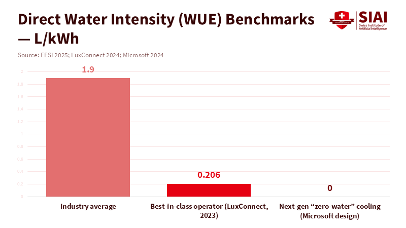
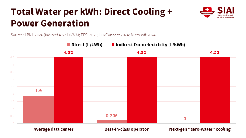
Operating a 100-megawatt AI campus for a year uses substantial water. The industry average for direct water use is about 1.9 liters per kWh, so cooling alone could take about 1.66 billion liters. Including the indirect water used to generate electricity—about 4.5 liters per kWh on a U.S. grid—the total exceeds 5 billion liters. This is a very important issue for communities and schools. Artificial Intelligence tutoring, learning analysis, and campus research all depend on computer power housed in data centers. How these data centers cool their systems determines if these benefits can grow without using up local water or causing power and heat problems for schools and cities. The choice is not between stopping new ideas and holding back, but between uncontrolled growth and planned growth. Education leaders can make rules for the systems they use more and more.
Data Center Water Cooling is Now an Education Issue
Education is quickly changing to Artificial Intelligence services. This change depends on a large increase in electricity use by data centers, which could double in a few years. Power usage has improved in some areas, but reducing electricity use does not eliminate heat. It only moves the problem to cooling. In hot, dry areas, many companies still use systems that evaporate water to save electricity, but this uses a lot of water. In cooler or wetter areas, they use chillers or liquid cooling to use less water, but these can use more power. School systems are stuck between two problems: higher power bills for services they now need, and political problems when a new computing center comes to town and uses a lot of water for data center cooling without telling people.
The other problem is trust. People in the community need to know how much water each facility uses directly and how much is used to generate power for the campus. Most companies do not clearly report both of these things, and even fewer promise to stay within a specific limit per unit of computer power. For schools, this means they are taking risks without control. Teachers want fast Artificial Intelligence tools, technology leaders want reliability, and facility teams want bills they can estimate. But the cooling methods and power sources behind these services are often kept secret. This gap will raise costs in the future. It also makes schools look bad if using Artificial Intelligence seems to be taking water away from the community.
Figure 1: Average data centers use ~1.9 L/kWh for cooling; best-in-class sites are near 0.2 L/kWh; next-gen designs target zero cooling water—set procurement at ≤0.4 L/kWh.
Design Rules: Data Center Water Cooling Without Local Harm
Education buyers can change things. They can make data center water cooling a key thing they ask about in every computer contract. They can set a water-use limit that decreases each year, and the limit is audited by an independent auditor. They can push to use 0.4 liters of water per kWh or less by the end of the decade, since some places are already close to zero water use. They can make companies share a water total that includes both direct cooling water and water used to generate electricity. This number should be easy to compare between different offers. They can also set a power-use limit near 1.1 to keep heat loss low. These two numbers—water use and power use—give schools a simple way to compare offers without getting lost in marketing.
Rules should go with buying. State education groups can create a computer budget rule: every new Artificial Intelligence program that uses the cloud must present a simple water-and-power plan. The plan should name the area where the data center is, the data center's cooling method, the expected water and power use, and how much of the energy is carbon-free, all day, every day. They can connect grant money to real-time reporting. They can make public dashboards so parents, teachers, and local leaders can see how much water and power are used each week for every thousand student actions. There is a give-and-take between electricity and water in cooling choices, but that should be clear. Once the numbers are easy to see, leaders can pick locations and sellers that fit local needs.
Figure 2: Even with “zero-water” cooling, electricity production adds ~4.5 L/kWh; cutting direct water from 1.9 to ~0 shrinks totals from ~6.4 to ~4.5 L/kWh.
Turning Heat to Learning: District Heating and Campus Wins
Computers make heat. When captured, that heat can warm homes, labs, and gyms. Some projects are showing how to do this on a big scale. Large projects in Nordic countries and Ireland take waste heat from server rooms, improve it with heat pumps, and send it to city networks. Universities are a good fit because they are near areas that need steady, low-temperature heat. They also control roofs, basements, and pipes where exchangers and pumps can be put. For a public university, a data center cooling plan that includes heat recovery is not just a bonus—it's a way to protect itself. It reduces winter gas use, keeps operating costs steady, and turns a negative into a positive for the public.
The design goal is simple: no wasted heat. Education buyers should ask in every cloud or colocation deal where the heat will go and who will benefit. If the facility is connected to district heating, it requires a signed agreement and a minimum annual heat delivery. If there is no network, ask for ways to use the heat on-site—such as hot water for dorms, pool heating, or greenhouse projects that support agriculture programs. Funding groups can prioritize grants that connect Artificial Intelligence programs to heat reuse. The costs are getting better as liquid cooling becomes more common. Liquid systems make it easier to capture heat at useful temperatures, reducing the size and cost of heat pumps. Schools can take charge by stating that the data center cooling plan includes a heat-recovery plan, not just a score for how well it performs.
From Mountains to the Sea: Data Center Water Cooling Beyond the City
Locations are changing. Some companies are moving computer operations to cooler mountain areas, where cold temperatures and cave-like tunnels lower cooling needs. Others are trying underwater modules that use the stable ocean conditions to remove heat without using freshwater. Another idea is still new but important: data centers in orbit that would use constant sunlight for power and the cold of space for cooling. None of these ideas is perfect. But they make the map bigger. For education, the lesson is clear. We should not assume that fast Artificial Intelligence must be close to the city. We should buy services that fit our climate and community needs, including the data center water cooling effects we are willing to accept.
These ideas do have trade-offs. Mountain tunnels and cool areas lower fan use and water needs, but they can be far from fiber networks, which adds network costs and delay. Underwater units avoid using freshwater and have proven reliable, but they face challenges with maintenance, permits, and seabed use. Space ideas promise clean power and easy heat removal, but launch pollution and space-junk risks must be reduced for them to help the climate. The policy for schools is not to pick one idea. It is to set goals. Ask sellers to meet strict water and power limits for each unit of computer power, and let them meet those limits with the mix of location and technology that works. If a company can meet the data center cooling standard under the sea, on a plateau, or in a park near a city heat network, that is their choice.
What Educators Should Do Next
Start with contracts. Every Artificial Intelligence tool used by schools should point to a computer center that meets public data center cooling and power standards. If a seller cannot show a water and power use number that can be checked, move on. Next, plan for the location. For tasks that can handle some delay—tests, model practices, data analysis—choose cooler, water-safe areas. For classroom tools that need to be fast, prefer locations that reuse heat into community networks. Then, connect payments to results. Make it cheaper for sellers to meet your standards than to avoid them. Offer long-term deals to providers that hit low-water and power-use levels and send heat into public or campus systems. Connect education technology renewal to lower use numbers each year. Share the results.
Build knowledge within your team. Train staff to understand water and power terms in data center contracts. Include in teacher and student training the link between Artificial Intelligence and these physical systems. Clearly define the key numbers: liters per kWh, watts per unit of compute, and megawatt-hours of heat reused. By making these numbers common knowledge, demand will drive the market toward better practices.
The first number is worth saying again. A year of computer use at a big Artificial Intelligence site can use billions of liters of water when you count both direct cooling and the water used for its power. That is not a reason to stop learning or researching. It is a reason to guide it. Schools are big buyers of digital services. They can require data center cooling that uses water, provides clean power, and recycles heat. They can pick locations that fit local water and energy limits. They can ask for clear information and turn down deals that hide the basics. If we want Artificial Intelligence in every class, we must count every liter and every kilowatt. The future we teach should be the one we make. Let education lead by setting the rules for the computer power it uses.
The views expressed in this article are those of the author(s) and do not necessarily reflect the official position of the Swiss Institute of Artificial Intelligence (SIAI) or its affiliates.
References
Aquatherm. (2025). Using waste heat from data centres: Turning digital heat into community warmth. Fortum. (2024). Microsoft X Fortum: Energy unites businesses and societies. Google. (2024). Power Usage Effectiveness. International Energy Agency. (2024). Electricity 2024—Executive summary. International Energy Agency. (2024). Energy and AI—Energy demand from AI. Lawrence Berkeley National Laboratory (Shehabi, A.). (2024). United States Data Center Energy Usage Report. LuxConnect. (2024). Water efficiency in the data center industry. Meta. (2020). Denmark data center to warm local community. Microsoft. (2024). Sustainable by design: Next-generation datacenters consume zero water for cooling. Microsoft. (2020). Project Natick: Underwater datacenters are reliable and conserve freshwater. Ramboll. (2024). Meta surplus heat to district heating. SEAI. (2023). Case study: Tallaght District Heating Scheme. Thales Alenia Space / ASCEND. (2024). Feasibility results on space data centers. UN Environment Programme—U4E. (2025). Sustainable procurement guidelines for data centres and servers. U.S. Department of Energy. (2024). Best practices guide for energy-efficient data center design. U.S. Environmental and Energy Study Institute. (2025). Data centers and water consumption. eGuizhou. (2024). How Guizhou’s computing power will drive fresh growth. China Daily. (2023). Tencent’s mountain-style data center in Gui’an. World Economic Forum. (2020). Project Natick overview. Reuters. (2025). Nordics’ efficient energy infrastructure ideal for Microsoft’s data centre expansion.
Picture
Member for
1 year 8 months
Real name
Catherine McGuire
Bio
Professor of AI/Tech, Gordon School of Business, Swiss Institute of Artificial Intelligence
Catherine McGuire is a Professor of Computer Science and AI Systems at the Gordon School of Business, part of the Swiss Institute of Artificial Intelligence (SIAI). She specializes in machine learning infrastructure and applied data engineering, with a focus on bridging research and large-scale deployment of AI tools in financial and policy contexts. Based in the United States (with summer/winter in Berlin and Zurich), she co-leads SIAI’s technical operations, overseeing the institute’s IT architecture and supporting its research-to-production pipeline for AI-driven finance.
Pivot Sanaenomics from populism to productivity
Protect real per-student spending and modernize vocational training
Target support, not handouts, to grow without tighter BOJ policy
Strengthen defence while protecting R&D and skills to keep growth alive
Spend smarter: joint procurement, open standards, and dual-use innovation
Fund what proves results—capability gains, cost declines, and real diffusion
Points-based immigration replaced EU free movement and filled shortages
Rapid rule swings now strain universities and care services
Use a public skills scorecard and align visas with training
AI That Seems Human: Rules and How They Affect Schools
Picture
Member for
1 year 9 months
Real name
Keith Lee
Bio
Keith Lee is Professor of AI and Finance at the Gordon School of Business, Swiss Institute of Artificial Intelligence (SIAI). His primary research lies in financial mathematics and AI-driven computational science, with a focus on quantitative modeling of complex economic and financial systems. His work integrates machine learning, stochastic modeling, and data-centric methods to study structural transformations in markets and institutions.
In recent years, his research has extended to the economic and fiscal implications of technological change, including the interaction between artificial intelligence, demographic shifts, and public finance sustainability.
He holds a PhD in Mathematical Finance from Boston University, and previously earned an MSc in Finance and Economics from the London School of Economics. He completed his undergraduate studies in Economics at Seoul National University under the Korea Foundation for Advanced Studies scholarship program.
He regularly contributes analytical essays on the broader socioeconomic implications of AI to The Economy Review.
Published
Modified
Human-like AI can blur boundaries for students in schools
Use clear identity labels, distance-by-default design, and distress safeguards
Align law, procurement, and classroom practice to keep learning human
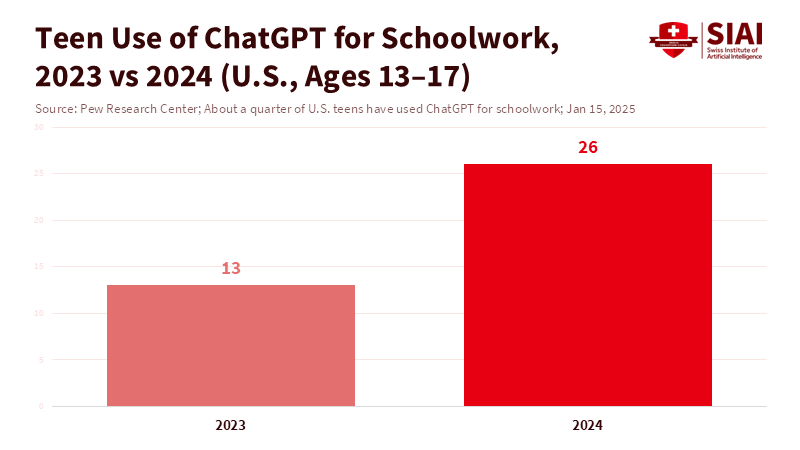
We often say present systems aren't thoughtful, but they can talk, listen, and comfort. So, schools, instead of tech blogs, will test how we should control AI that seems human. One thing to remember is that in 2025, around 25% of teens in the U.S. said they used ChatGPT for school, which is up from about half that number the year before. It's being accepted quickly and used often without people realizing it. When a tool can sound like a classmate, a tutor, or a mentor, it's hard to tell what's what. If the goal of AI rules is to prevent people from confusing humans and machines, then education is where it matters most. Grades, input, and trust depend on knowing who is who. We don't want to ban better tools. We want to keep learning humans while making AI safer, more trustworthy, and less like a person, mainly when a student is feeling lonely.
Why AI Rules Matter in Schools
The need for AI rules in schools stems from a core risk: students can easily confuse responsive, friendly chatbots for people, especially when seeking comfort or help. Even if a tool is not truly sentient, it can still influence effort, trust, and emotional support—key building blocks in education. The threat lies not in AI thinking like people, but in seeming to care like them. Clear rules are necessary to maintain educational standards and safeguard student well-being.
Some recent rules are aimed at the biggest problems. Draft rules in China would regulate AI that behaves like people and forms emotional connections, with rules to warn about excessive use, flag when someone is upset, and reduce loyalty. The Science Press says these rules might affect matters outside China. Thinking about schools shows why. Students often use AI alone at home late at night. Even if schools have rules, things change faster than those rules can keep up. A clear, easy rule—don't act like a human; don't try to make friends; always label machine identity—gives leaders and sellers the same plan. It also offers teachers words they can use in class without having to know the law very well. If leaders stay focused on that, AI rules become a helpful tool rather than a barrier to improvement.
Figure 1: Teen use of ChatGPT for schoolwork doubled in one year, making disclosure and distance-by-default urgent for schools.
What Students Are Doing
Data on who uses these programs shows a clear truth. Saying We don't use it here doesn't work anymore. Surveys in 2025 found that around 26% of U.S. teens used ChatGPT for school, up from 13% in 2023. More people are using it, with one measure in mid-2025 saying that about one-third of adults have used it. Younger adults were the first to start. Other surveys show that the most common use is still looking for info and generating ideas, but using it for business is higher among people under 30 than among older people. Basically, the classroom and teens are where voice, tone, and seeming caring are most likely to be felt.
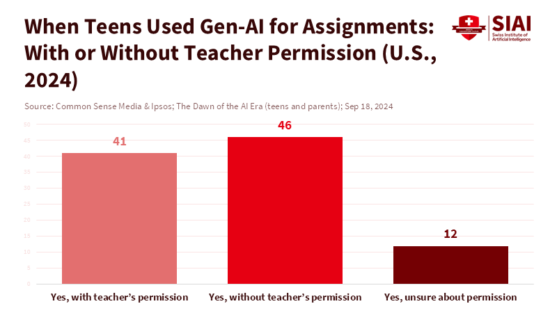
Figure 2: Many teens who use gen-AI for assignments do so without teacher permission, underscoring the need for clear classroom rules and provenance.
School data tells another story. Many parents know these tools exist, but not enough get clear help from schools. Teens say rules change from teacher to teacher and from class to class. Some students have had their work wrongly marked as AI-generated. That hurts trust. It also makes students want to write like a machine to avoid being improperly marked. AI rules fix this mess. If systems must say they are machines and not act like humans, schools can shift from looking for rule-breakers to planning. They can pick tools that show how they work. They can set assignments that need steps to be checked. And they can help students when they might use AI for comfort instead of learning.
The hardest proof is also the most human. News reports have highlighted problematic situations that prompted the leading platforms to add parental controls and teen-safety features. No one case makes a policy. But enough is happening to treat loyalty and sadness as the main risks. In education, where most users are young, we need to set the bar high. AI rules put the bar in the tool, not just in the school policy book. If a tool can tell that a teen account is being used a lot late at night, it should slow down. If it hears signs of harm, it should point away from talking openly to checked, small answers and clear, human help lines. These aren't parts of intelligence. They are parts of design.
Design for Distance: Make AI Less Human, More Helpful
The goal is to build distance without losing help. That's the design idea behind AI rules. Make the system say who it is — always—in text, voice, and picture, so there's no question. Keep a normal tone in voice mode. Use words that suggest a tool, not a friend. Don't give first-person info that sounds like a story. Don't use flirty or parental words with young people. Need noticeable watermarks in what's on the screen and what's heard. And stop long, caring talks when sadness is found, replacing them with short, helpful prompts and ways to reach trained people.
Adding the classroom changes three things. First, thinking about tests. When a student opens a quiz or an assignment in a learning system, AI support should switch to help mode. That means hints, examples, and questions that make you think with citations, not complete answers. The tool shows how it works and keeps the student in charge. Second, where things come from is normal. What is made should include explain buttons that go to sources, thinking steps, and the model version. That lets teachers judge use, not guess it. Third, agreed rules for young people. Linked parent-teen accounts can set quiet hours, limit session lengths, and block voice messages that sound like those from friends or teachers. These options should be easy to get, not special.
Sellers will say these limits hurt their chances of being accepted. The opposite is more likely in education. Tools that keep a clear line between help and copying build trust with the areas and parents. They also lower legal risk. Narrowing how you sound lowers the risk that a tool becomes a late-night friend instead of a study friend. Nothing here needs a perfect telling of feelings or plans. It needs normal settings, visible identity signs, and slowdown triggers when usage exceeds simple limits.
From Doubts to Safety Measures: A Policy Path
We started with doubt: if current systems aren't truly thoughtful, do AI rules do anything? In education, the answer is yes. The issue isn't what's inside the model. It's what's seen on the outside. Seeming warmth and being there, at a high level, can act like a person when it matters. So policy should mix three things—law, buying, and practice—that make distance stronger by design.
In law, keep AI rules focused and clear. Ban copying specific people. Need to be told the machine identity at all times. Don't allow emotional-bond parts for young people. Order slow-down and out when distress signals are seen. Insist on checkable records of these things, kept with strong privacy. These items align well with current international drafts and can be incorporated into local rules.nto local rules.
When buying, areas should buy based on how things act, not just on skill. Ask sellers to say they can prove three items: identity signs that can't be turned off; youth-safety buttons that can be made normal; and where things come from, which makes classroom use possible. An AI rules list can be included in every request for proposal. Over time, that market sign will matter more than any one policy paper.
In practice, schools should change tasks so that AI is there but kept in check. Use talks, journals, and whiteboarding to connect learning to how things are done. Teach students to ask with citations and to write down how an AI suggestion changed their work. Replace complete bans with staged use: brainstorming allowed, writing limited, final writing personal. These moves are old teaching with a new reason. They work better when the tool is made to act like a tool.
The likely concern is that all this will stop getting better and hurt support. But the goal isn't to make AI improve its capabilities in ways that reduce mistaken closeness. In education, clarity helps learning. We can make systems better at math and calmer at writing while keeping them clearly not human. That's the deep point of AI rules. They are about keeping the human parts of school—judgment, care, and responsibility—by stopping the machine from acting like a friend or a mentor.
The first thought said these rules were empty because today's AI isn't human. The classroom shows the problem. Students react to tone and timing, not just to truth. A machine that sounds patient at 1 a.m. can pull a teen into long talks that feel. We can't forget that risk as acceptance increases. Once gets higher. The better way is to keep the help and lower the guessing. AI rules do that by making distance part of the product and the policy at once. If we label identity, stop acting like a persona, slow in sadness, and prove where things come from, we keep learning in human hands. The policy goal isn't to win a discussion about intelligence. It's to protect students while raising standards for proof, writing, and care. That's why doubt should give way to safety measures. In schools, we should want AI that's more right, more helpful, and clearly not us. The AI rules that many once ignored may be the easiest way to get there.
The views expressed in this article are those of the author(s) and do not necessarily reflect the official position of the Swiss Institute of Artificial Intelligence (SIAI) or its affiliates.
References
AP-NORC Center for Public Affairs Research. (2025). How U.S. adults are using AI. Cameron, C. (2025). China’s plans for human-like AI could set the tone for global AI rules. Scientific American. Common Sense Media & Ipsos. (2024). The dawn of the AI era: Teens, parents, and the adoption of generative AI at home and school. Pew Research Center. (2025a). About a quarter of U.S. teens have used ChatGPT for schoolwork. Pew Research Center. (2025b). 34% of U.S. adults have used ChatGPT. Reuters. (2025). China issues draft rules to regulate AI with human-like interaction. Time. (2025). Amid lawsuit over teen’s death by suicide, OpenAI rolls out parental controls for ChatGPT.
Picture
Member for
1 year 9 months
Real name
Keith Lee
Bio
Keith Lee is Professor of AI and Finance at the Gordon School of Business, Swiss Institute of Artificial Intelligence (SIAI). His primary research lies in financial mathematics and AI-driven computational science, with a focus on quantitative modeling of complex economic and financial systems. His work integrates machine learning, stochastic modeling, and data-centric methods to study structural transformations in markets and institutions.
In recent years, his research has extended to the economic and fiscal implications of technological change, including the interaction between artificial intelligence, demographic shifts, and public finance sustainability.
He holds a PhD in Mathematical Finance from Boston University, and previously earned an MSc in Finance and Economics from the London School of Economics. He completed his undergraduate studies in Economics at Seoul National University under the Korea Foundation for Advanced Studies scholarship program.
He regularly contributes analytical essays on the broader socioeconomic implications of AI to The Economy Review.