The Economic Cost of War: Why Lost Labor and Capital Crush Recovery
War slashes output by destroying labor and capital
Ukraine’s displacement and ruined infrastructure cause long, Europe-wide economic scars
Recovery hinges on safe returns, demining, and rebuilding power and transport to unlock investment

Rebuilding the Center: Multicultural Education Policy for a Changing Australia
Australia’s diversity is high; classrooms decide cohesion
Data show immigrant students succeed with language support and safe schools
Priorities: rapid language screening, teacher training, and clear cohort tracking
Australia is
Algorithmic Decoupling Will Change What U.S. Students See Online
U.S. spin-off narrows feeds
Students lose global views
Mandate diversity metrics, open datasets

TikTok reaches millions of Americans every day, and a significant number are students. In 2024, Pew found that 58% of U.S.
The AI Cognitive Extensions Gap: Why Korea’s Test-Prep Edge Won’t Survive Generative AI
The AI Cognitive Extensions Gap: Why Korea’s Test-Prep Edge Won’t Survive Generative AI

Catherine McGuire is a Professor of Computer Science and AI Systems at the Gordon School of Business, part of the Swiss Institute of Artificial Intelligence (SIAI). She specializes in machine learning infrastructure and applied data engineering, with a focus on bridging research and large-scale deployment of AI tools in financial and policy contexts. Based in the United States (with summer/winter in Berlin and Zurich), she co-leads SIAI’s technical operations, overseeing the institute’s IT architecture and supporting its research-to-production pipeline for AI-driven finance.
Published
Modified
Korea excels at teen “creative thinking,” but adults lag in adaptive problem solving
Generative AI automates routine tasks, so value shifts to AI cognitive extensions—framing, modeling, and auditing
Reform exams, classroom routines, and admissions to reward those extensions, or the test-prep edge will fade

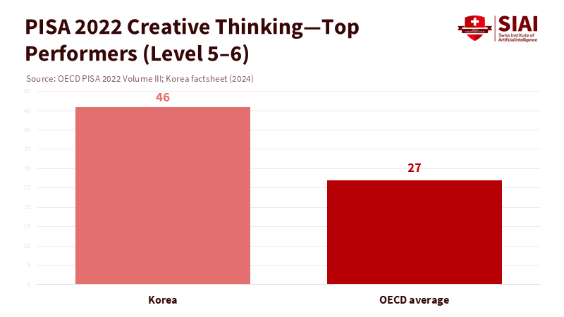
Fifteen-year-olds in Korea excel in “creative thinking.” In 2022, 46% reached the top levels on the OECD test, well above the OECD average of 27%. However, Korean adults struggle with flexible, real-world problem-solving. On the OECD Survey of Adult Skills, 37% score at or below Level 1 in adaptive problem solving, and only 1% reach the top level. This gap is significant. School-age achievements in "little-c" creativity do not translate into adult skills in defining problems, synthesizing evidence, and designing solutions alongside AI. Generative tools speed up this change. Randomized studies show that AI improves routine writing quality by about 18% and reduces time spent by around 40%. Customer support agents solve 14-15% more queries with the help of AI. The real value lies in the human steps before and after automation—what we term AI cognitive extensions: scoping, modeling, critiquing, and integrating across sources. Systems that depend heavily on algorithmic training will struggle, while those that teach AI cognitive extensions will thrive.
AI Cognitive Extensions: Paving the Way for a New Era in Education
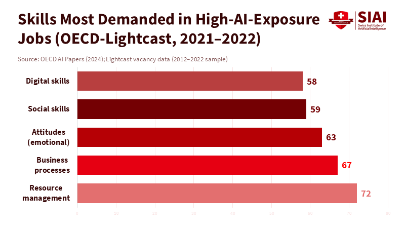
Generative AI now takes on much of the execution work that schools have valued: standard writing, template coding, routine data transformations, and procedural math. In 10 OECD countries, jobs most affected by AI already prioritize management, collaboration, creativity, and communication. Seventy-two percent of high-exposure job postings require management skills, and demand for social and language skills has increased by 7-8 percentage points over the past decade. As tools handle more tasks, employers appreciate the ability to set up the task, break down challenges, evaluate outputs, and communicate decisions across teams. These are AI cognitive extensions. They are not mere soft skills; they represent crucial judgment skills in a world where basic tasks are automated.
Korea has been moving in this direction on paper. The 2022 national curriculum revision, a comprehensive update to the educational framework, aims to cultivate “inclusive and creative individuals with essential skills for the future,” with a focus on uncertainty and student agency. However, policy intent faces cultural challenges. Private after-school tutoring remains nearly universal and is optimized for high-stakes exams. In 2023-2024, participation was around 78-80%, and spending reached record levels—about ₩27-29 trillion—despite a declining student population. The education system still rewards algorithmic speed under exam pressure. This system cannot deliver AI cognitive extensions at scale.
What the Data Says About Korea’s Strengths—and Weak Links
It is tempting to say the system is already succeeding based on high PISA scores in creative thinking. But a closer look reveals the truth. PISA measures' little-c' creativity in familiar contexts for 15-year-olds, assessing the ability to generate and refine ideas within set tasks. It does not evaluate whether graduates can define tasks themselves, combine evidence from different fields, or check an AI's reasoning under uncertainty. The picture changes for adult skills. Korea’s average literacy, numeracy, and adaptive problem-solving in the PIAAC survey fall below OECD averages, with a notably thick lower range in adaptive problem-solving. This discrepancy creates labor-market challenges, such as a mismatch between the skills students possess and the skills employers need, which schools pass to universities and employers. It also highlights the need for AI cognitive extensions.
AI adoption further emphasizes the importance of framing over mere execution. Randomized studies show that generative tools improve output for routine writing and standard customer support, especially for less-experienced workers on templated tasks. Coding experiments with AI pair programmers exhibit similar time savings. Automation reduces the value of algorithmic execution, the very area that cram schools optimize. The emphasis shifts to individuals who can write effective prompts, define evaluation criteria, blend domain knowledge with statistical insight, and justify decisions in uncertain situations. Essentially, AI handles more of the “show your work” aspect, and humans must decide which work to present initially. This is the gap Korea needs to bridge.
Designing an AI Cognitive Extensions Curriculum
The solution lies in the curriculum, not superficial tweaks. Start by teaching students the tasks that AI cannot easily manage: defining problems, selecting evaluation measures, and justifying trade-offs. Make these actions clear. In math and data science, the shift from just solving problems to discussing “model choice and critique”: why choose a logistic link over a hinge loss; the significance of priors; where confounding variables might hide; and how we would identify model drift. In writing, revise assessments from finished essays into decision memos that include evidence maps and counterarguments. In programming, replace bland problem sets with “spec to system” tasks where students must gather requirements, create basic tests, and then use AI to draft and refine while documenting risks. These practices introduce AI cognitive extensions as a series of habits that can be assessed for quality and reproducibility.
Korea can move quickly because its education system already rigorously tracks performance. Substitute some timed, single-answer tests with short, frequent tasks where students submit: a problem frame, an AI-assisted plan, an audit of their model or tool choice, and reflections on their failures. Rubrics should evaluate the clarity of assumptions, the choice of evaluation metrics, and the student’s ability to highlight second-order effects. This approach maintains meritocratic standards while rewarding advanced thinking. National curriculum language that emphasizes adaptable skills allows for such shifts; the challenge is effectively applying those changes in schools still influenced by hagwon culture. Adjusting classroom incentives to promote AI cognitive extensions is essential for turning policy into practice.
The institutional evidence is telling. A selective European program that imported Western, problem-based AI education into Asia found that a large majority of its Asian students struggled to apply theory to open-ended applications and synthesis. This prompted a redesign of admissions and teaching methods. The issue was not a lack of mathematical ability; instead, it highlighted the missing connection between abstract concepts and real-world applications in uncertain situations—the very essence of AI cognitive extensions. While one case can’t replace national data, it shows how quickly high-performing test takers can stumble when tasks change from executing algorithms to creating them. We should view this as a cautionary tale and a guide for improvement.
Accountability That Rewards AI Cognitive Extensions
Assessment must evolve if curricula are going to change. The national exam system offers a straightforward opportunity for reform. Korea’s test reforms have primarily focused on removing “killer questions.” While this may reduce the competition in private tutoring, it does not assess what truly matters. Instead, introduce scored components that cannot be crammed for: scenario briefs with uncertain data, brief oral defenses of plans, and audit notes for an AI-assisted workflow that flag hallucinations, biases, and alignment risks. Assess these using double-masked rubrics and random sampling to ensure fairness and scalability. If the exam rewards AI cognitive extensions, the system will teach them.
The second area for change is teacher practices. Recent studies of curriculum decentralization show that just giving teachers more freedom does not ensure improvements; they need practical tools and shared routines. Provide curated task banks aligned with the national curriculum’s goals, along with examples of problem framing, evaluation design, and AI auditing. Pair this with quick-cycle professional learning that reflects student tasks; teachers should practice writing prompts, setting acceptance criteria, and conducting red-team reviews. When teachers have heavier workloads, AI should assist with routine paperwork to free up time for coaching higher-order skills. This approach makes AI cognitive extensions a real practice rather than just a slogan.
Lastly, align signals in higher education. Universities and employers should favor admissions and hiring practices that look for portfolios showcasing framed problems, annotated code and data notes, and decision documents with clear evaluation criteria. Analysis of Lightcast data across OECD countries shows growing demand for creativity, collaboration, and management in AI-related roles. Suppose universities publish criteria that require these materials. In that case, secondary schools will start teaching them, and this time it will be effective. Building a strong connection between signals and skills is how Korea can maintain its excellence and update its competitive edge.
The headline figures tell different stories: Korea’s teenagers shine in tested creativity, but many adults struggle with adaptive problem-solving in real-world situations. Generative AI sharpens this divide. It automates much of the task's core and shifts value to the beginning and end: the framing at the start and the audit at the end. These edges constitute AI cognitive extensions. They can be taught, assessed fairly, and scaled when exams, classroom activities, and higher education signals support them. Maintain algorithmic fluency; it still has its place. However, do not mistake fast computation under pressure for the ability to define problems, manage uncertainty, and guide tools with sound judgment. The path forward is not to slow down or ban AI in classrooms. Instead, it involves making the human aspects of the work—the parts that guide AI—visible, regular, and graded. If we act now, Korea can turn its early-stage creative strengths into adult capabilities. If we don’t, students who were prepared for yesterday’s challenges will see their advantages fade. The decision—and the opportunity—are ours.
The views expressed in this article are those of the author(s) and do not necessarily reflect the official position of the Swiss Institute of Artificial Intelligence (SIAI) or its affiliates.
References
Bae, S.-H. (2024). The cause of institutionalized private tutoring in Korea. Asia Pacific Education Review.
Brynjolfsson, E., Li, D., & Raymond, L. (2025). Generative AI at Work. Quarterly Journal of Economics, 140(2), 889–951.
Brynjolfsson, E., Li, D., & Raymond, L. (2023). Generative AI at Work (NBER Working Paper No. 31161).
Lightcast & OECD. (2024). Artificial intelligence and the changing demand for skills in the labour market. OECD AI Papers.
Noy, S., & Zhang, W. (2023). Experimental evidence on the productivity effects of generative artificial intelligence. Science.
OECD. (2023). PISA 2022 results (Volumes I & II): Korea country notes.
OECD. (2024). PISA 2022 results (Volume III): Creative thinking—Korea factsheet.
OECD. (2024). Survey of Adult Skills (PIAAC) 2023 Country Note—Korea and GPS Profile: Adaptive problem solving.
Peng, S., et al. (2023). The impact of AI on developer productivity. arXiv:2302.06590.
Seoul/Korean Ministry of Education; Statistics Korea. (2024–2025). Private education expenditures surveys. (News summaries and statistical releases).
SIAI (Swiss Institute of Artificial Intelligence). (2025). Why SIAI failed 80% of Asian students: A Cognitive, Not Mathematical, Problem. SIAI Memo.
UNESCO. (2023). Guidance for generative AI in education and research.
Catherine McGuire is a Professor of Computer Science and AI Systems at the Gordon School of Business, part of the Swiss Institute of Artificial Intelligence (SIAI). She specializes in machine learning infrastructure and applied data engineering, with a focus on bridging research and large-scale deployment of AI tools in financial and policy contexts. Based in the United States (with summer/winter in Berlin and Zurich), she co-leads SIAI’s technical operations, overseeing the institute’s IT architecture and supporting its research-to-production pipeline for AI-driven finance.


Cashless by Design, Resilient by Default: Digital Money Resilience for Schools and Universities
Schools must plan for digital money resilience as payments go cashless
Keep layered rails—fast digital by default, cash and offline modes for outages
Pilot CBDC/stablecoin use with strict safeguards, contracts, and treasury diversification

Pacific Climate Education Is the Missing Pillar of Island Resilience
Climate finance must fund people, not just projects
Put Pacific climate education at the center
Tie every grant to learning-days and local ownership

In a year when the oceans in the South-West Pa
Rethinking AI Energy Demand: Planning for Power in a Bubble-Prone Boom
Rethinking AI Energy Demand: Planning for Power in a Bubble-Prone Boom

David O’Neill is a Professor of AI/Policy at the Gordon School of Business, SIAI, based in Switzerland. His work explores the intersection of AI, quantitative finance, and policy-oriented educational design, with particular attention to executive-level and institutional learning frameworks.
In addition to his academic role, he oversees the operational and financial administration of SIAI’s education programs in Europe, contributing to governance, compliance, and the integration of AI methodologies into policy and investment-oriented curricula.
Published
Modified
AI energy demand may surge—but isn’t guaranteed
Nuclear later; near-term: renewables, storage, shifting
Schools should plan for boom or bust with flexible procurement

By 2030, global electricity generation for data centers is expected to exceed 1,000 TWh, about double 2024 levels and nearly 3% of total global electricity generation. This figure is significant. It reflects both the scale of growth in computing and a deeper tension in policy. If we view AI energy demand as fixed and unavoidable, we risk embedding today's hype into tomorrow's power systems. However, this scenario isn't predetermined. Demand will depend on how quickly models are used, business adoption, and profit margins that justify ongoing expansion. If growth slows or if the AI bubble deflates, projections that assume steady increases will be off target. If growth persists, we may struggle to provide enough clean power quickly. Either way, educators, administrators, and policymakers should not rely solely on averages; they must create adaptable strategies to prepare for both increases and decreases.
The United States serves as a stress test. An assessment supported by the U.S. Department of Energy predicts that data centers will grow from approximately 4.4% of U.S. electricity use in 2023 to between 6.7% and 12% by 2028, driven by AI adoption and efficiency gains. BloombergNEF estimates that meeting AI energy demand could require 345 to 815 TWh of power in the U.S. by 2030, translating to a need for 131 to 310 GW of new generation capacity. These estimates vary widely because the future is genuinely uncertain. They depend on factors such as usage rates, inference intensity, cooling technology, and hardware advancements. This uncertainty should inform public investment and campus procurement strategies: plan for peaks while being prepared for plateaus.
The standard narrative is straightforward: AI chips consume a lot of power, cloud demand is increasing, and grids are under pressure; thus, we must expand clean power, particularly nuclear energy. This chain of reasoning holds some truth but is incomplete. The missing element is the conditional nature of demand. Much of the anticipated load growth relies on business models—such as autonomous systems taking over many white-collar jobs—that haven't yet proven effective at scale. If those assumptions don't hold, the story about AI energy demand shifts from a steep rise to a plateau. Our goal is to create policies for energy and education that apply to both potential outcomes, avoiding the pitfalls of excessive optimism or pessimism.
Productivity Claims vs. Power Reality
Evidence on productivity in specific situations is encouraging. In a significant field study, providing a generative AI assistant to over 5,000 customer support agents increased the number of issues resolved per hour by about 14% on average, with greater gains for less experienced staff. This indicates real improvements at the task level. However, this alone does not prove that automated systems will replace a large share of jobs or maintain the high inference volumes needed to ensure rapid growth in AI energy demand through 2030. Overall productivity is essential because it funds capital expenditures and keeps servers operational. In 2024, U.S. non-farm business labor productivity grew by about 2.3%. This is good news, but it isn't just about AI, nor is it enough to provide a substantial change to settle the energy debate.
Macroeconomic signals are mixed. Analysts have highlighted a notable gap between the capital expenditures for AI infrastructure and current AI revenues. Derek Thompson and others summarize estimates suggesting spending on AI-related data centers could reach $300 to $400 billion by 2025, compared to much lower current revenues—typical indicators of a speculative boom. Even some industry leaders acknowledge bubble-like traits while emphasizing the necessity for a multi-year runway. If revenue growth falls short, usage will shift from exponential to selective, leading to a decline in AI energy demand. This possibility should be considered in grid and campus planning—not as a prediction, but as a scenario with specific procurement and contracting consequences.
The baseline for data centers is also changing rapidly. The International Energy Agency (IEA) projects that global electricity consumption by data centers could double to about 945 TWh by 2030, growing roughly 15% per year, which is over four times the growth rate of total electricity demand. U.S. power agencies anticipate a break from a decade of flat demand, driven in part by AI energy needs. However, the IEA also highlights significant differences in the sources of new supply: nearly half of the additional demand through 2030 could be met by renewables, with natural gas and coal covering much of the rest, while nuclear energy's contribution will increase later in the decade and beyond. This mix highlights the policy dilemma: should we aim for slower demand growth, faster clean supply, or both?
Nuclear's Role: Urgent, but Not Instant
Nuclear power has clear advantages for meeting AI energy demand: high capacity factors, stable output, a small land footprint, and life-cycle emissions comparable to those of wind power. In 2024, global nuclear generation reached a record 2,667 TWh, with average capacity factors around 82%. This reliability is valuable to data center operators. These attributes are crucial for long-term planning. The challenge lies in time. Recent data indicate that median construction times range from approximately 5 to 7 years in China and Pakistan, to 8 to over 17 years in parts of Europe and the Gulf, with some western projects taking well beyond a decade. Small modular reactors, often touted as short-term solutions, have faced cancellations and delays; the flagship project in Idaho was terminated in 2023. In other words, while nuclear is a strategic asset, it alone cannot handle the immediate surge in AI energy demand.
This timing issue is significant because the period from 2025 to 2030 is likely to be critical. Even optimistic timelines for small modular reactors suggest that the first commercial units won't be ready until around 2030; many large reactors now under construction will not connect to the grid before the early to mid-2030s. Meanwhile, wind and solar energy sources are being added at unprecedented rates—around 510 GW of new renewable capacity in 2023 alone—but their variable generation and connection backlogs limit how much of the AI surge they can support without storage and transmission improvements. The practical takeaway is a three-part plan: push for nuclear expansion in the 2030s, accelerate renewable energy and storage investments now, and implement demand-side strategies to manage AI energy demand in the meantime.
Even in a nuclear-forward scenario, careful procurement matters. Deals for data centers near campuses should combine long-term power purchase agreements with enforceable clean-energy guarantees, not just claims about the grid mix. Where nuclear is feasible, offtake contracts can support financing; where it is not, long-duration storage and reliable low-carbon options—including geothermal and hydro updates—should form the basis of the energy strategy. The goal of policy is not to choose winners, but to secure reliable, low-carbon megawatt-hours that align with the hourly demands of AI energy.
What Schools and Systems Should Do Now
Education leaders are in a unique position: they are significant electricity consumers, early adopters of AI, and trusted community conveners. They should respond to AI energy demand with three specific actions. First, treat demand as something that can be shaped. Model the load under two scenarios: ongoing AI-driven growth and a moderated rate if automated systems don't deliver. Align procurement with both scenarios—short-term contracts with flexible volumes for the next three years, and longer-term clean power agreements that expand if usage proves sustainable. Include provisions to reduce usage during peak times, and implement price signals that encourage non-essential tasks to be done during off-peak hours. This same approach should apply to campus research groups: establish scheduling and queuing rules that prioritize daytime solar energy whenever possible and enhance heat recovery from servers for buildings.
Second, connect education to energy use. Update curricula to specify AI energy demand within computer science, data science, and EdTech programs. Teach energy-efficient model design, including quantization, distillation, and retrieval, to reduce inference costs. Introduce foundational grid knowledge—such as capacity factors and marginal emissions—so graduates can develop AI that acknowledges physical limits. Pair this learning with real-world procurement projects: allow students to analyze power purchase agreement terms, claims of additionality, and hourly matching. Future administrators will need this knowledge as much as they require skills in privacy or security.
Third, plan for both growth and decline. If usage skyrockets as anticipated, the U.S. could need between 11% and 26% more electricity by 2030 to support AI computing; campuses should prepare to adjust workloads, invest in storage, and strengthen distribution networks. If the bubble bursts, renegotiate the minimum terms of offtake agreements, direct surplus clean energy toward electrifying fleets and buildings, and retire the least efficient computing resources early. Taking these approaches safeguards budgets and supports climate goals. It is crucial to reject the notion that the only solution is to produce more energy. Good policy must also address demand.
Anticipating the Strongest Critiques
One critique suggests that efficiency will outpace demand. New designs and improved power utilization effectiveness (PUE) could limit AI energy needs. This is a plausible argument. However, history warns of the Jevons paradox: lower costs per token can lead to increased consumption. Even the most positive efficiency projections indicate that overall demand will still rise in the IEA's base case, as user growth outweighs savings from improved efficiency. Others argue that AI could offset its energy costs through enhanced productivity. Studies at the task level show gains, particularly among less experienced workers, and U.S. productivity has improved. Yet, these advancements are not substantial enough at this point to guarantee the revenue streams necessary to support permanent, exponential growth. It is wiser to plan for different possible outcomes, rather than deny potential issues.
A second critique argues that nuclear energy can meet the rising demand if we "choose to build." We should indeed make that choice—quickly and safely. However, current timelines present challenges. Recent global construction times vary greatly; early adopters of small modular reactors have faced setbacks, and large projects in the West continue to have extensive delays. While nuclear is necessary in the mix for the 2030s, it is not a quick fix for AI energy demands in 2026. This is why procurement strategies must combine short-term renewable and storage solutions with long-term firm sources. Regulators must also expedite transmission and interconnection processes; without proper infrastructure, new clean energy resources cannot reach new demand.
A third critique argues that fears of an "AI bubble" are exaggerated. This may be true. However, even industry insiders recognize bubble-like characteristics in the market while suggesting that any downturn may still be years away. For public institutions, the appropriate response is not to stake everything on either scenario. Instead, they should ensure flexibility: secure adaptable contracts, staged developments, colocated storage, and systems that maximize value from every kilowatt-hour. This strategy works well in both growth and downturn periods.
Design for Uncertainty, Not For Averages
The key numbers are concerning. Global AI energy demand for data centers could surpass 1,000 TWh by 2030. In the U.S., AI could account for 6.7% to 12% of total electricity by 2028, and meeting growth needs by 2030 could require adding 131 to 310 GW of new capacity. These estimates validate the need for urgent action without leading to despair. They also remind us to stay humble about what the future holds: if automated systems fail to generate substantial productivity consistently, usage will decline, and long-term energy investments based on steady growth will fall short. Conversely, if AI continues to expand, every clean megawatt we can create will be essential, with nuclear energy playing a more significant role later in the decade and into the 2030s. The unifying theme is design. Institutions should approach AI energy demand as a variable they can control—shaped through contracts, software, education, and operations. This involves securing flexible offtake today, investing in robust low-carbon supply tomorrow, and maintaining a constant focus on efficiency. It also means graduating students who understand how to work with the existing grid and the new grid we need to build. The call to action is clear: prepare for growth, protect against downturns, and ensure that every incremental terawatt-hour is cleaner than the last.
The views expressed in this article are those of the author(s) and do not necessarily reflect the official position of the Swiss Institute of Artificial Intelligence (SIAI) or its affiliates.
References
BloombergNEF. (2025, October 7). AI is a game changer for power demand.
Brynjolfsson, E., Li, D., & Raymond, L. (2023). Generative AI at Work (NBER Working Paper No. 31161).
Ember. (2025, April 8). Global Electricity Review 2025.
IEA. (2024–2025). Energy and AI: Energy demand from AI; Energy supply for AI.
IEA. (2024). Electricity 2024 – Executive Summary.
IEA. (2023). Renewables 2023 – Executive Summary.
LBNL/DOE. (2024, December 20). Increase in U.S. electricity demand from data centers. U.S. DOE summary.
Reuters. (2025, February 11). U.S. power use to reach record highs in 2025 and 2026, EIA says.
U.S. BLS. (2025, February 12). Productivity up 2.3 percent in 2024.
World Nuclear Association. (2024–2025). World Nuclear Performance Report; capacity factors and 2024 generation record.
World Nuclear Industry Status Report. (2024). Construction times 2014–2023 (Table).
Thompson, D. (2025, October 2). This Is How the AI Bubble Will Pop.
The Verge. (2025, Aug.). Sam Altman says "yes," AI is in a bubble.
Business Insider. (2025, Oct.). Former Intel CEO Pat Gelsinger says AI is a bubble that won't pop for several years.
David O’Neill is a Professor of AI/Policy at the Gordon School of Business, SIAI, based in Switzerland. His work explores the intersection of AI, quantitative finance, and policy-oriented educational design, with particular attention to executive-level and institutional learning frameworks.
In addition to his academic role, he oversees the operational and financial administration of SIAI’s education programs in Europe, contributing to governance, compliance, and the integration of AI methodologies into policy and investment-oriented curricula.
Counting the Uncounted: Pricing Climate Spillover Costs in Advanced Economies
Climate spillover costs spread climate damage across borders and supply chains, not just disaster zones
Standard models miss these externalities, so budgets and prices understate true risk
Measure and price spillovers to fund resilience in education and public services now

Policy Uncertainty, Not Polarization, Explains Spain's Talent Squeeze
Policy uncertainty, not polarization, drives Spain’s talent loss
Low vacancy rates and selective outflows show thin, unreliable opportunities
Fix it with stable multi-year funding and fixed calendars to lift hiring

Spain entered 2025
How Education Can Break China’s Rare Earth Monopoly
China’s rare earth monopoly sits in midstream refining and magnet production, not mines
An education-led push—rapid training, teaching factories, and industry-linked research—builds the workforce to shift capacity
Procurement, recycling, and allied coordination then cut risk faster than tariffs alone