Thickening the Shield: Why Europe Must Accept a Profit Hit for Stronger AT1 Capital
Europe must thicken AT1 capital buffers even if it permanently lowers bank profits
Digital bank runs make thin hybrid capital unreliable in real stress
Clear, equity-like AT1 design is cheaper than repeated public rescues

Wearable AI: How Our Bodies Are Becoming the Next Tech Hub
Wearable AI is moving computing from screens to body-level devices
Education policy must balance personalization with privacy and trust
Early rules will decide whether wearable AI helps learning or harms it

Initially, artificial intelligenc
The Next Binding Frame: Rebuilding Order When the Rules-Based Order Frays
The rules-based order is breaking into competing systems
Asia is building regional frameworks to manage the shift
Education and institutions must adapt to fragmented governance

The international system we've relied on for dec
Rebuilding Ukraine: Why the Korea 1953 Template is Useful — but Not Enough
Ukraine cannot rely on the 1990s transition model without rebuilding core infrastructure
The Korea 1953 case shows why catalytic capital must target hard assets first
A phased Ukraine reconstruction strategy is key to unlocking private investment and EU integration

Freedom, Skills, and Growth: Why Human Capital and Democracy Must Be Recast as a Joint Project
Democracy raises growth most where human capital is already strong
Freedom and skills act as multipliers, not substitutes, in economic development
Sustained prosperity requires joint investment in institutions and people

Pay for the Light: Why AI transparency funding must be the price of openness
Pay for the Light: Why AI transparency funding must be the price of openness

In recent years, his research has extended to the economic and fiscal implications of technological change, including the interaction between artificial intelligence, demographic shifts, and public finance sustainability.
He holds a PhD in Mathematical Finance from Boston University, and previously earned an MSc in Finance and Economics from the London School of Economics. He completed his undergraduate studies in Economics at Seoul National University under the Korea Foundation for Advanced Studies scholarship program.
He regularly contributes analytical essays on the broader socioeconomic implications of AI to The Economy Review.
Published
Modified
AI transparency is a public good that cannot survive without explicit funding
Unfunded openness will weaken Western firms against state-subsidized competitors
Paying for transparency is the only way to keep AI markets both open and competitive

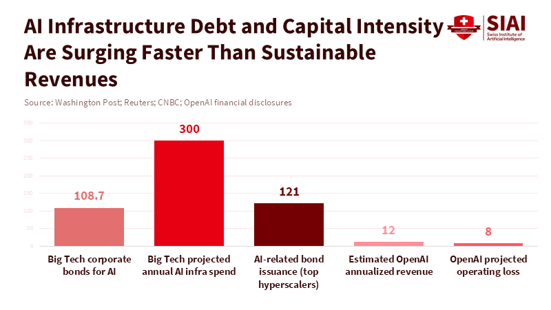
In the last three months of 2025, tech companies borrowed around $109 billion through corporate bonds to pay for the intense competition in AI. Big AI companies shifted from small research budgets to huge data centers and computing power, costing them tens of billions more. This shows something important: open AI systems will only stay open if there's money to cover the electricity, staff, checks, and responsible management that make openness real. Saying that AI transparency is a good thing, legally or morally, is important, but it's not the whole story. According to the California State Legislature's Transparency in Frontier Artificial Intelligence Act, new regulations require companies developing artificial intelligence to increase transparency, which could create challenges for international competitors, especially those backed by governments. To protect both our values and fair competition, we have to connect transparency with a way to pay for it. This AI transparency funding would put a fair price on the benefits to everyone and treat funding as a clear part of policy.
The Reality of Paying for AI Transparency
First, a lot of money is being spent on infrastructure. Top companies are building massive data centers and borrowing a lot to do it. Teaching and running the biggest AI models now needs constant money for computer chips, power, cooling systems, and fast connections. Companies get this money from investors, partners, and by selling bonds. This creates a pattern: investors are paying for growth now, hoping to make money later. But making money later isn't a sure thing. Competition, increased efficiency, and global politics can lower the expected profits. Open AI models and shared training data increase costs because of checks, removing sensitive info, paperwork, and following rules. This doesn't directly create new income unless it's used to make money. This creates a common problem: companies are asked to provide something good for everyone – real transparency – but their own profits depend on keeping their technology secret.
Second, there's a big difference in government support around the world. Many AI projects in China get direct and indirect support from the government. This includes money, tax breaks, shared computer networks, and support from local governments, which lowers the cost for companies to grow. According to the Foreign Policy Research Institute, local governments in China, such as in Beijing, Shanghai, and Shenzhen, subsidize the cost of computing power for AI startups through computing power vouchers. In contrast, companies in the United States generally do not receive similar government support. This matters because if transparency rules are the same for everyone, without considering where the money comes from, it could favor companies that are supported by subsidies. If transparency is a requirement for everyone, it needs to come with different ways to pay for it, or it will unfairly hurt companies that don't get subsidies.
That's why AI transparency funding is important: we need to pay for transparency directly. This could be done in different ways, like:
- Direct payments from the government to help companies check their AI.
- A fee paid by big AI companies that goes into a fund for public transparency.
- Tax credits for independent checks of AI models.
- Payments to smaller companies to help them follow the rules.
The specific plan is important, but the main idea is simple. If transparency creates benefits for everyone – like less misinformation, better safety, ways for regulators to check AI, and more trust – then it makes sense to use public money or have the industry work together to pay for it. Asking companies to pay for it on their own puts a strain on the market and encourages them to cut corners.
AI Transparency Funding: How to Compete with Rivals Supported by Governments
The central strategic question for Western firms is not whether transparency is desirable — it is — but how to keep their commercial engines running while meeting it. Open models and published datasets can create ecosystem value: researchers reuse, startups build, regulators inspect. But monetising that value is nontrivial. Advertising, enterprise subscriptions, vertical services and device ecosystems are plausible revenue routes for companies steeped in platform economics. Yet the numbers show a gap between headline valuations and durable cash flow in many frontier players, and the capital intensity of data centres and chips keeps growing. That gap is why some investors speak of an “AI bubble”: valuations price in sustained, very large margins that hinge on monopoly positions or unmatched scale. When rivals are state-backed, the contest is not just about product quality; it is about who can afford to subsidise a long investment horizon.
A practical response is to design transparency rules that recognise financing realities. One element is transitional relief calibrated by firm size, revenue, or access to strategic capital. Another is co-funding arrangements that link transparency to commercial advantage: firms that open crucial model documentation could receive preferential access to public procurement, tax credits for AI R&D, or co-funded compute credits. That makes transparency a serviceable investment — companies will open up because it buys market access and lowers other costs. A second element is mandatory contribution models. If the public gains from independent audits, a small industry levy earmarked for public-interest auditing bodies can scale as the market grows; that prevents free-riding and keeps audit capacity well-funded.
A final element is targeted risk sharing for the costliest pieces of transparency: independent red teams, third-party compute replication for validation, and long-running model documentation. These are expensive, uncertain, and not easily amortised into a subscription fee. Pooling those costs, or underwriting them through public guarantees, reduces the chance that a firm will avoid transparency because it cannot afford the verification.
AI Transparency Funding: Principles for Design and Policy
Policy should be based on four connected ideas. First, transparency requirements should be clear and specific. If they're vague, companies will do the minimum. Specify what information to share (model cards, training data, computer budgets, audit logs) and how to make results reproducible. Second, fund the standards. Create a public group to check AI, funded by user fees, industry fees, and government money, to avoid being controlled by companies. Third, match requirements to capabilities. Very large models that can do many things should have stronger transparency and cost-sharing requirements than small, specialized models. This allows for new ideas while targeting the biggest risks.
Fourth, make funding depend on performance. Payments, credits, and contracts should go to companies that meet strict transparency goals, checked by independent auditors. This sends a message that transparency isn't just for show, but a performance measure that improves competitiveness. It also avoids punishing companies that are transparent but underperform. Funds should reward real openness and verifiability. For small companies, the costs of auditing and paperwork make it harder for the rule to enter the market.
A good plan could use different ways to support transparency. A basic transparency standard would apply to all systems used widely. According to a study by Theresa Züger, Laura State, and Lena Winter, evaluating AI projects with a public-interest and sustainability focus can involve funding mechanisms such as a fee that increases with revenue to support public audits and measures to monitor computing power. Additional payments could be allocated to shared resources that benefit everyone, including safety test datasets, open benchmarks, and independent studies that assess how AI models perform. International cooperation would help create a level playing field. If foreign subsidies are clear, trade solutions or similar funding could be considered to prevent unfair advantages. The policy should involve laws, funding, and international agreements.
AI Transparency Funding: What It Means for Educators, Administrators, and Policymakers
Educators and administrators need to see AI transparency funding as both something to manage and something to teach. For universities and research labs, transparent funding can be a way to have steady collaboration. Government or industry payments that require open model documentation create predictable income for staff and data management. Administrators should develop the ability to manage data and audit models in the long term. These skills will be valuable in both education and public service. When buying AI systems, education systems should prefer companies that commit to real transparency and accept cost-sharing or payment plans tied to audit performance.
For policymakers, the challenge is to create the right system. Short, simple rules will either be avoided or create too many burdens. Instead, create a policy that combines basic requirements, shared funding, and targeted rewards, using many tools. Create clear ways to report information and to obtain third-party certification to reduce problems. Most importantly, build public audit groups with technical knowledge and shared governance so they can't be easily controlled by companies. Internationally, coordinate standards with other countries so that transparency requirements don't unfairly hurt companies.
Expect some criticism. Some will say that public funding of transparency is helping companies too much. The response is that the public already pays when private systems create problems like misinformation, privacy issues, and systemic risk. Funding transparency is an investment that reduces those problems and creates a public asset: models and datasets that can be audited and checked. Others will argue that fees and requirements will stop new ideas. But history shows the opposite when rules are paired with predictable funding and market rewards. Clarity lowers uncertainty and can grow markets by building trust. Finally, some will say that supporting domestic companies is protectionist. That's why the plan is important: link support to auditability and provide access to shared public resources, and allow qualified international companies to participate under similar rules.
Transparency without funding is just talk. The huge sums being spent on AI development show why funding is important. If openness is going to be real, it has to be priced and funded in a way that protects competition, encourages verification, and protects the public interest. Policymakers should create AI transparency funding now. They should fund public audit groups, allow fees tied to company size, and create benefits for verified openness. Educators and administrators should demand suppliers that can be audited and build the ability to manage models. Investors should prefer companies that see transparency as an asset. If we do this, openness will become a competitive advantage. If we don't, transparency will either be fake or cause companies to leave the market. We have a choice to make, and time is running out.
The views expressed in this article are those of the author(s) and do not necessarily reflect the official position of the Swiss Institute of Artificial Intelligence (SIAI) or its affiliates.
References
Bloomberg. (2026). A guide to the circular deals underpinning the AI boom. Bloomberg Business.
Epoch AI. (2025). Most of OpenAI’s 2024 compute went to experiments. Epoch AI Data Insights.
Forbes. (2025). AI data centers have paid $6B+ in tariffs in 2025 — a cost to U.S. AI competitiveness. Forbes.
Financial Times. (2025). How OpenAI put itself at the centre of a $1tn network of deals. Financial Times.
Rand Corporation. (2025). Full Stack: China's evolving industrial policy for AI. RAND Perspectives.
Reuters. (2026). OpenAI CFO says annualized revenue crosses $20 billion in 2025. Reuters.
Statista. (2024). Estimated cost of training selected AI models. Statista.
Visual Capitalist. (2025). Charted: The surging cost of training AI models. Visual Capitalist.
Washington Post. (2026). Big Tech is taking on more debt than ever to fund its AI aspirations. Washington Post.
CNBC. (2025). Dust to data centers: The year AI tech giants, and billions in debt, began remaking the American landscape. CNBC.
In recent years, his research has extended to the economic and fiscal implications of technological change, including the interaction between artificial intelligence, demographic shifts, and public finance sustainability.
He holds a PhD in Mathematical Finance from Boston University, and previously earned an MSc in Finance and Economics from the London School of Economics. He completed his undergraduate studies in Economics at Seoul National University under the Korea Foundation for Advanced Studies scholarship program.
He regularly contributes analytical essays on the broader socioeconomic implications of AI to The Economy Review.


Japan Silk Road Diplomacy
Japan is positioning governance as an alternative to China’s infrastructure power
AI rules and institutions are emerging as tools of geopolitical influence
Central Asia’s autonomy will hinge more on standards than on concrete

The great unspoken rate shock: why “silent tightening” was never silent
Silent tightening was not silent — it reshaped global credit through hidden market channels
Geopolitical shocks shifted capital from venture funding to private credit, slowing growth
The real policy failure is ignoring how financial plumbing redirects risk

When Data Skips a Key Variable: Rethinking femicide drivers in Europe
Femicide risk is misread when key population variables are left out
Missing data distorts which policies appear to work
Better models are needed to target prevention effectively

Here's something that should make us rethink o
The Case for Continuing DOGE’s Disruption — Reframing Federal AI Adoption
The Case for Continuing DOGE’s Disruption — Reframing Federal AI Adoption

Ethan McGowan is a Professor of AI/Finance and Legal Analytics at the Gordon School of Business, SIAI. Originally from the United Kingdom, he works at the frontier of AI applications in financial regulation and institutional strategy, advising on governance and legal frameworks for next-generation investment vehicles. McGowan plays a key role in SIAI’s expansion into global finance hubs, including oversight of the institute’s initiatives in the Middle East and its emerging hedge fund operations.
Published
Modified
Federal AI adoption depends on tools and training, not elite titles
DOGE proved rapid automation can work but exposed skill gaps
Lasting reform requires institutionalized AI, not rollback

Getting AI into the federal government isn't about finding rare AI geniuses. It's more about giving regular people the right tools and boosting everyone's basic skills across a huge system. When tools that write drafts, make summaries, and clean up data become available to workers, the key thing isn't having amazing AI models. Instead, it's about whether people can actually use these tools well in their daily jobs. The last year showed both the good and bad sides of this idea. There was a quick rollout of tools for agencies, but also a lot of public worker changes. This worried some people, but the big lesson is obvious: trying to fit people into specific job titles misses the point. What really matters is setting up these tools, helping everyone learn to use them, and ensuring workers have a reason to adopt the new, more productive ways of doing things. That's why it's important to keep pushing forward with DOGE's efforts to modernize, even if we need to fix some mistakes along the way.
Why federal AI adoption must be driven by tools, not titles
When it comes to AI in the federal government, success should be measured by how many useful systems are in use, not by how important the people who used to sit in fancy offices are. The government has been putting AI assistants to work in offices, which is having a real impact. Instead of just writing research papers, these tools are being tested by groups and early users. This shows that AI is more likely to be accepted when workers see how it helps them every day - like writing an email, summarizing a document, or automating a form. It's not just about adding a research scientist to the organization chart. This means changing the way we think, from hiring people with only knowledge to putting AI capabilities directly into how people work. It can be messy and reveal where skills are lacking, but it's the only way to ensure the public gets the most out of AI.
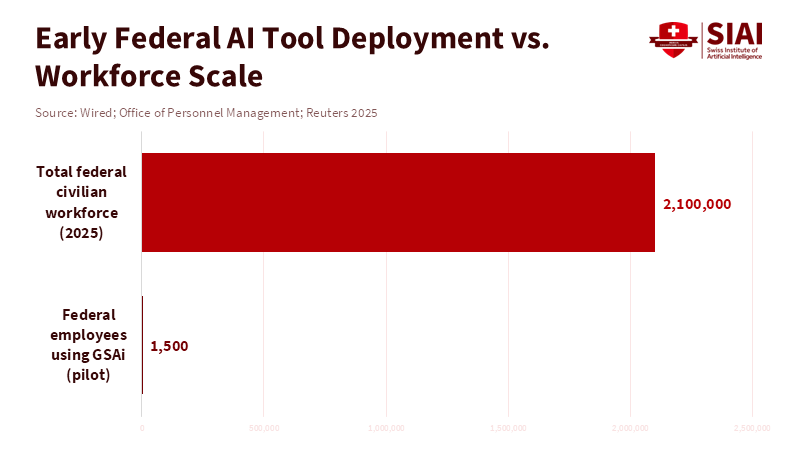
Using automated tools changes the number of people needed for different jobs. While some routine jobs become less necessary, there's a greater need for new roles, such as trainers, prompt engineers, data managers, support specialists, and people who ensure everything is done correctly. These jobs aren't the same as doing academic AI research, and it's a mistake to mix the two. If they're seen as the same, agencies might hire too many people with rare skills or fail to spend enough on the support needed to turn AI models into services people can rely on. According to WIRED, DOGE has taken steps to support regular federal workers in using AI tools by deploying its proprietary GSAi chatbot to 1,500 employees at the General Services Administration. This doesn't mean we can ignore ethics, safety, and oversight. Instead, it means that the people who create the rules and the people who understand the technology need to work together. They need to turn safety rules into practical guidelines that staff can follow. Having clear rules for handling data, simple checklists, and automatic logging makes people feel less afraid and makes it easier to try new things. Focusing on practical guidelines rather than creating fancy job titles will make AI adoption in the federal government something that lasts, rather than just for show.
How DOGE's Actions Moved AI Forward
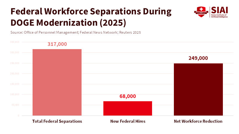
DOGE's focus on quick changes had a clear result: AI assistants were rolled out into everyday work, and there were big reductions in the number of employees, which made news. According to the Office of Evaluation Sciences, about 35 percent of GSA employees used the agency's internal GenAI chat tool at least once within the first five weeks after it launched, suggesting that while these systems can assist with daily tasks, a significant portion of workers may not be adopting them immediately. According to a report from Federal News Network, when agencies automated certain tasks, it removed the need for people to handle time-consuming manual work, allowing staff to concentrate on more strategic responsibilities. This led to improvements in efficiency but also brought significant changes to how people worked.
At the same time, the number of workers changed a lot. Reports showed that many people left their jobs during this period. This explains why adopting AI felt difficult: the people who knew the old ways of doing things and could help make the transition were often the ones leaving. This doesn't mean trying to modernize was a mistake. It means we need a clearer, slower plan to keep important knowledge while introducing new tools. We need to recognize that automation reduces some work, but knowledge is still needed to make sure technology is used safely and effectively.
Finally, public arguments about who was fired and why mixed politics with misunderstandings about technology. Some people left because they were still in a trial period or because their jobs were really software engineering roles labeled as research. According to a recent article, there remains confusion in public administration over the distinction between AI researchers and those skilled in statistical modeling or software implementation. However, the article emphasizes that modernizing with AI is necessary, provided that related vulnerabilities are carefully managed. It's to make job definitions clearer and invest in retraining workers. This way, people with implementation skills can move into jobs that support and monitor automated systems, rather than just being replaced.
Training for the Future
If the goal is to have AI widely and safely used in the federal government, the first step is to improve basic skills across agencies. This means funding affordable training for many employees on how to use AI assistants daily, write effective prompts, spot errors, and keep data clean. Training should be hands-on, short, and focused on specific tasks, not just abstract workshops on how models work. When training is practical, people are more likely to use AI because they see the direct benefits. This approach treats tools and users as equally important: neither can succeed without the other. Investing in training is much cheaper than replacing entire teams and prevents the loss of knowledge that happens when experienced people leave.
In practice, agencies should provide support when rolling out new tools. Every test should include specialists who can fix prompts, document problems, and create simple reports that show where the assistant is helpful and where it isn't. These specialists don't need to be experts; they just need to understand how things work, relate to people, and have some technical skills. By creating these middle-skill positions, the government makes the transition smoother and creates career paths for existing staff. This makes adopting AI more inclusive.
Another good idea is to introduce automation step by step. Instead of sudden layoffs and full-scale replacements, agencies should automate specific tasks, check them against human review, and then expand. This reduces the chance of errors and keeps human judgment where it's important. It also creates a series of successes that build support. The lesson is simple: speed without support creates problems, but speed with support leads to lasting change.
Making it Last
To make AI adoption in the federal government successful long-term, policymakers should focus on three things: tools, training, and governance. Procurement and certification should favor usable solutions that come with strong support and clear plans for how to fit them into existing systems. This means looking beyond the AI model itself and requiring user training, built-in security, and post-deployment monitoring. Workforce policy should fund quick re-skilling programs and create clear career paths for the middle-skill jobs that keep automation running smoothly. This prevents confusion between researchers and engineers from leading to long-term talent shortages. Governance should be practical, with required logging, regular audits, and easy-to-use systems for reporting incidents that nontechnical staff can use. These three pillars will make AI adoption in the federal government sustainable, no matter who is in charge.
Some might worry about fairness, accuracy, and how fast things are changing. They might say that quick automation leads to mistakes and hurts public services. They are right to ask for safeguards. The answer isn't to slow everything down, but to demand clear safety measures before expanding: error rates under human review, the number of sensitive data incidents, and how confident users are. These measures can be achieved and enforced when tests are designed to produce them. Taking a “measures-first” approach turns abstract ethical concerns into practical “pass/fail” checks that protect the public while allowing useful systems to grow.
Finally, the question of people leaving their jobs needs to be addressed clearly. If people left mostly on their own or are still in a trial period, steps can be taken to keep the knowledge of those who remain: creating written guides, recording walkthroughs, and offering short periods for departing staff to transfer their knowledge. If people were fired unfairly, legal and HR solutions should be used. But neither situation is a reason to reject modernization. The goal is to balance speed with care, so AI adoption improves services.
AI adoption in the federal government is most successful when it is practical, responsible, and builds skills. DOGE's actions put pressure on companies to put tools in workers' hands and show what automation can do. The mistakes made, such as cutting staff too quickly, not defining jobs clearly, and not providing enough training, can be fixed. By combining deployments with training, rolling out automation step by step, and creating clear rules, we can secure gains while preserving important knowledge. If the goal is to improve services, policymakers should keep pushing for modernization. The goal is to put usable tools in people's hands, teach them to use them safely, and build a system that lasts. That is how AI adoption becomes a real improvement that citizens can see, measure, and trust.
The views expressed in this article are those of the author(s) and do not necessarily reflect the official position of the Swiss Institute of Artificial Intelligence (SIAI) or its affiliates.
References
Brookings Institution. “How DOGE’s modernization mission may have inadvertently undermined federal AI adoption.” January 21, 2026.
Politico. “Pentagon’s ‘SWAT team of nerds’ resigns en masse.” April 15, 2025.
Reuters. “DOGE-led software revamp to speed US job cuts even as Musk steps back.” May 8, 2025.
Wired. “DOGE Has Deployed Its GSAi Custom Chatbot for 1,500 Federal Workers.” March 2025.
U.S. Office of Personnel Management. Federal workforce data, personnel actions and separations (2025 updates). 2025–2026 dataset.
ZDNet. “Tech leaders sound alarm over DOGE’s AI firings, impact on American talent pipeline.” March 2025.
Ethan McGowan is a Professor of AI/Finance and Legal Analytics at the Gordon School of Business, SIAI. Originally from the United Kingdom, he works at the frontier of AI applications in financial regulation and institutional strategy, advising on governance and legal frameworks for next-generation investment vehicles. McGowan plays a key role in SIAI’s expansion into global finance hubs, including oversight of the institute’s initiatives in the Middle East and its emerging hedge fund operations.