Low-Cost Automatic Detection of Board Channel-Induced Failures in Semiconductor Testing based on Channel-Sharing Test Boards

1. Introduction

1.1. Problem Description

In semiconductor manufacturing, testing is an indispensable process to verify the functional and electrical characteristics of manufactured products, thereby screening out defective units and ensuring that only high-quality products reach the market. Since the efficiency of this testing process directly correlates with productivity, cost, and market competitiveness, reducing test time and cost remains a continuous challenge in the industry [1]. Against this background, parallel testing, a method for testing multiple semiconductor products simultaneously, has become a standard practice.

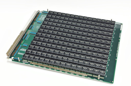
One of the representative test apparatus used for parallel testing is test board, a physical example of which is shown in Figure 1. Hundreds of Devices Under Test (DUT) are mounted onto a test board in a grid-like array, allowing for their simultaneous test within a single test cycle and dramatically reducing overall test time. To further enhance testing efficiency, semiconductor manufacturers developed channel-sharing test boards, which routes electrical signals for testing to multiple DUTs through a single shared channel. They enable increasing test throughput with fewer channels, economizing the costly test channels while significantly improving the efficiency of the testing process. Consequently, channel-sharing architecture is widely employed, particularly in the memory and general-purpose system semiconductor testing fields where cost competition is intense.

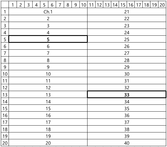
However, this efficient architecture leads to a peculiar and challenging type of false failure, hereafter referred to as Board Channel-Induced Failure (BCIF). This issue is largely due to physical impairments accumulated through repeated test executions, including mechanical wear or micro-cracks of connectors and sockets, which degrade the signal integrity of the shared channel. If such a defect occurs in a specific channel, all DUTs connected to it are erroneously classified as failures, regardless of their actual operational status. For instance, if channels 5 and 33 in the layout shown in Figure 2 are defective, the corresponding DUTMAP, a data representation of test results for each DUT coordinate on the test board, will exhibit a distinct pattern where all DUTs belonging to those channels are marked as failures, as illustrated in Figure 3. Such defective board channels causes the misclassification of potentially good products as failures, consequently decreasing the manufacturing yield and increasing the average production cost.

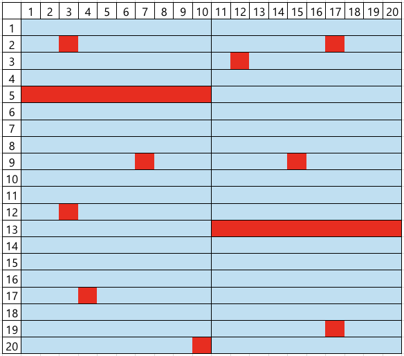
To address this issue, engineers in practice perform a manual re-classification by visually inspecting the DUTMAP to identify BCIFs. This work is based on a heuristic inference: if there are some channels where all DUTs are marked as failures while the overall failure rate of the DUTMAP is low, they are considered as BCIFs. This reasoning is predicated on the logic that such a spatial pattern of failures is improbable to occur without underlying channel faults. Conversely, as shown in Figure 4, if the overall background failure rate is high, the complete failure in a channel could plausibly be a coincidental result, which is insufficient evidence to declare BCIFs. Based on this judgment, DUTs suspected of BCIF are scheduled for a re-test on the other test board, affording them a chance to be salvaged as good products rather than scrapped. In contrast, other failed DUTs are scrapped to avoid the additional costs and process delays associated with re-testing.

However, this manual work suffers from several intrinsic limitations. First, it is a labor-intensive task that demands the attention of engineers. Second, the time required for this manual inspection can become a bottleneck, impeding overall test process. Third, the reliance on a qualitative judgment of whether such a spatial pattern is `improbable' introduces subjectivity and inconsistency, as different engineers may apply different criteria. Therefore, there is a pressing need for an automated system to replace this manual re-classification. This necessitates the development of methods to detect whether BCIFs exist in the observed DUTMAP in real-time with high accuracy, so as to improve both the efficiency and yield of semiconductor testing based on channel-sharing test boards.

1.2. Related Work

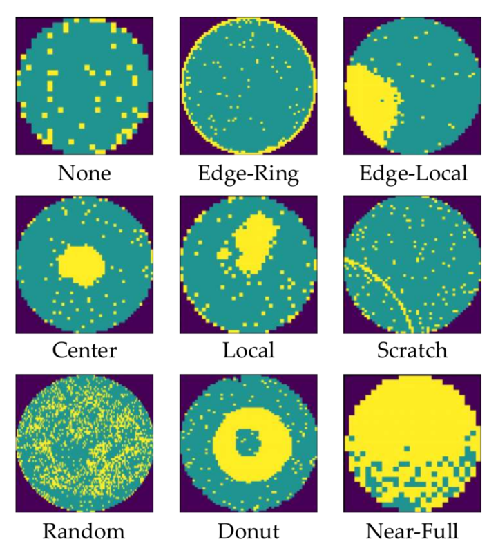
Numerous studies have focused on detecting spatial anomalies in semiconductor test 'map', which is a data representation of coordinate-wise test results such as DUTMAP, using machine learning. In particular, research on wafermap (see Figure 3), which display the test results of individual chips on a wafer, has been actively conducted. While these studies differ in methodological details, many share a common approach of using Convolutional Neural Networks (CNNs) to learn and detect spatial defect patterns within wafer maps [2]. In contrast, research on DUTMAP is comparatively scarce. The method introduced in the patent by [3] is the most relevant prior work to the BCIF detection problem addressed in this study, which also employs a CNN to learn spatial defect patterns in DUTMAPs for anomaly detection.

However, these supervised learning-based approaches present several challenges for practical application in industrial settings, which are also pertinent to the BCIF detection problem. First, training deep learning models incurs significant costs associated with acquiring and operating expensive GPU machines. Second, the process of collecting samples and labeling them for a dataset demands substantial effort of engineers in the field. This issue is particularly acute for BCIF detection because a single dataset is insufficient. The spatial pattern of BCIFs, such as the one shown in Figure 4, is contingent on a specific channel layout like that in Figure 2. Since different test boards may have varying channel layouts, the resulting BCIF patterns also change. Consequently, a new dataset must be prepared each time a test board with a new channel layout is introduced. Third, manual labeling is prone to errors, which adversely affects model performance. For instance, when presented with Figure 4, one engineer might label it as a non-BCIF DUT map based on the logic described in Section 1-1. Problem Description, while another might label it as a BCIF. One of these is a labeling error, and a high frequency of such errors will degrade the model's performance as it learns from flawed data.

2. Proposed Methodology

In order to being free from three issues above, we propose an methodology which requires no model training process. This methodology is based on statistical hypothesis testing, and we call it Channel Defect Test (CDT). The core idea is to compute the likelihood ratio between the observed DUTMAP under the 'channel defects' hypothesis versus the 'nomal' hypothesis.

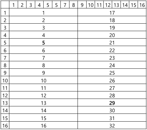
To formulate the test, we begin by mathematically representing the board's channel layout and the DUT failure occurrence structure depending on the presence or absence of channel defects. Representing test board and channels as index sets of their constituent DUTs, the entire board can be expressed as ${1, \ldots, N}$, and the channels as its partitions $C_1, \ldots, C_M$. Taking Figure 2 as an example, the entire board region ${1, \ldots, 20 \times 20}$ is partitioned into 40 channels $C_1, \ldots, C_{40}$. Individual test results of DUTs are represented by variables $x_n \in {0, 1}$ for $n=1, \ldots, N$, where $0$ denotes pass and $1$ denotes fail. The region of channels where all DUTs failed, such as channels 5 and 33 in Figure 2-1, and the region of the other channels are denoted by

• $A = \bigcup_{x_n = 1, \forall n \in C_m} C_m \text{ and } A^c = {1, \ldots, N} - A,$

respectively.

Our Goal is to judge whether the observed $A$ is a probabilistic coincidence even in the absence of defective channels, or a structural phenomenon resulting from underlying channel defects. For this purpose, we first model the test results of DUTs as

• $x_n \sim \text{Bernoulli}(p_n), \text{ where } p_n = \begin{cases} p_A & \text{for } n \in A \ p_{A^c} & \text{for } n \in A^c \end{cases}, $

$p_A$ and $p_{A^c}$ denote the failure probabilities in $A$ and $A^c$, respectively. In practice, DUTs on a single board are homogeneous products with identical components and manufacturing processes, so we assume they have the equal intrinsic failure probability. CDT tests the following two competing hypotheses for $p_A$ and $p_{A^c}$, which can be interpreted as whether $A$ represents a region of defective channels:

• $H_0: p_A = p_{A^c} = p_0 \in (0, 1)$
• $H_1: p_A = 1, \, p_{A^c} = p_1 \in (0, 1)$

$H_0$ states that the failure probability in $A$ is not different to that in $A^c$, meaning the observed $A$ is just a probabilistic phenomenon. Conversely, under $H_1$, $A$ represents an area where DUTs fail with probability 1, indicating it is the region of defective channels. These two competing perspectives are intuitively illustrated in Figure 6 and Figure 7, respectively. Rejection of $H_0$ leads to the detection of all DUTs within $A$ as BCIFs, which are then scheduled for re-testing.

We derive the test statistic of CDT based on Likelihood Ratio Test (LRT) framework. Under $H_0$, the observed $A$ and the number of failures in $A^c$, denoted as $\tilde{x} = \sum_{n \in A^c} x_n$, are the result of failures occurring with probability $p_0$ across the entire board region. Therefore, the resulting likelihood function under $H_0$ is

• $Binomial(|A|; |A|, 1) \times Binomial(\tilde{x}; |A^c|, p_1)$ - Equation 1

The multiplicative form of the two $Binomial$ functions stems from the fact that events occurring in $A$ and $A^c$ are independent, which is a direct consequence of the physical isolation between channels.
The maximum likelihood estimators for $p_0$ and $p_1$ are their respective sample failure rates [5]: $\hat{p}_0 = \dfrac{|A| + \tilde{x}}{|A| + |A^c|}$ and $\hat{p}_1 = \dfrac{\tilde{x}}{|A^c|}$. By substituting these estimators into the likelihood functions, we can derive the likelihoods ratio as

• $LR(|A|, |A^c|, \tilde{x}) = \dfrac{Binomial(|A|; |A|, \hat{p}_0) \times Binomial(\tilde{x}; |A^c|, \hat{p}_0)}{Binomial(|A|; |A|, 1) \times Binomial(\tilde{x}; |A^c|, \hat{p}_1)} = \hat{p}_0^{|A|} \left( \dfrac{\hat{p}_0}{\hat{p}_1}\right)^{\tilde{x}} \left(\dfrac{1 - \hat{p}_0}{1 - \hat{p}_1}\right)^{|A^c| - \tilde{x}} - \text{Equation 2}$

Finally, we define the test statistic of CDT as the negative log-likelihood ratio, $T(|A|, |A^c|, \tilde{x}) = -\log LR(|A|, |A^c|, \tilde{x})$. Then $H_0$ is rejected if $T(|A|, |A^c|, \tilde{x})$ exceeds a predefined critical value.

3. Experimental Results

This section presents simulation studies designed to validate the performance and robustness of the proposed methodology CDT and to demonstrate its practical superiority over the supervised CNN learning. The Data Generating Process (DGP) for the DUTMAP is based on several realistic assumptions.

1. While all DUTs share a intrinsic failure probability, those within a defective channel are guaranteed to fail.
2. The number of defective channels and the intrinsic failure probability of the product vary depending on the test board's condition and the product's characteristics.
3. The location of these defective channels and individual failures is random rather than structurally determined.

In essence, the DGP of a DUTMAP is determined by a combination of two parameters: the number of defective channels and the intrinsic DUT failure probability. For a given pair, a DUTMAP is generated as follows. First, $d$ channels are randomly selected from the total channels $C_1, C_2, \ldots, C_M$, and their union is defined as the defective region $D$, with the remaining area being $D^c$. Subsequently, the test result for each DUT, $x_n$, is generated from a conditional Bernoulli distribution:

• $x_n \sim \text{Bernoulli}(p_n) \text{ for } n = 1, \ldots, N, \text{ where } p_n = \begin{cases} 1 & text{for } n \in D \\ p_{D^c} & \text{for } n \in D^c \end{cases}$

All simulations assume a test board with a channel layout commonly used in the industry, as depicted in Figure 8, where $N = 256$ and $M = 32$.

3.1.Simulation 1: Performance Comparison with a Conventional Method under Realistic Scenarios

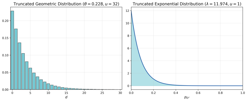
The first simulation aims to compare the performance and its stability of CDT and a CNN-based approach under a parameter distribution that mimics real-world manufacturing conditions. We assume $d$ follows a truncated geometric distribution with an upper limit $u = 31$ and a rate parameter $\theta = 0.2283$, pmf of which is denoted as $TruncGeo(d; \theta = 0.2283, u = 31)$. This reflects the reality that the probability of having no defective channels ($$d=0$$) is highest, and it decreases exponentially as the number of defective channels increases. $p_{D^c}$ is assumed to follow a truncated exponential distribution with an upper limit $u = 1$ and a rate parameter $\lambda = 11.9741$, pdf of which is denoted as $TruncExp(p_{D^c}; \lambda = 11.9741, u = 1)$. This captures the observation that the intrinsic failure probability is typically close to $0$ and the probability diminishes as it approaches $1$. The rate parameters for both distributions were set based on internal private data from Samsung Electronics, and their pmf and pdf are visualized in Figure 9. Since the intrinsic product failure probability and the number of board defects are independent, their joint distribution function is the product of their individual distribution functions:

• $f(d, p_{D^c}) = TruncGeo(d; \theta = 0.2283, u = 31) \times TruncExp(p_{D^c}; \lambda = 11.9741, u = 1)$

Then DUTMAPs without channel defects, labeled as $y=0$, are generated from $f(d, p_{D^c} | d = 0)$, while those with channel defects, labeled as $y=1$, are generated from $f(d, p_{D^c} | d > 0)$. The experiment consists of 200 independent simulation runs. In each run, we generate datasets for training (10,000 DUTMAPs), validation (2,000 DUTMAPs), and testing (2,000 DUTMAPs), ensuring a balanced 50:50 class ratio for the presence of channel defects, $y$. Performance is evaluated using the $F_1$-Score on the test dataset.

Layer (Activation)	Output Shape	Parameters
Input	(16,16,1)	0
Channel-wise Convolution (ReLU)	(16,2,2)	18
Max Pooling	(2,2,2)	0
Flatten	(8)	0
Fully Connected (ReLU)	(3)	27
Output (Sigmoid)	(1)	4
Total parameters: 40

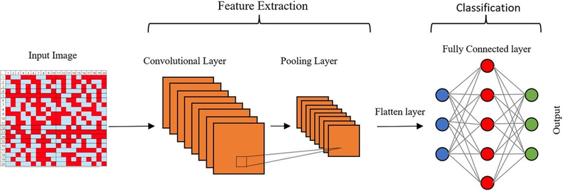
The comparative CNN model employs a simple architecture, as shown in Figure 10 and detailed in Table 1, which is a simplified version of typical small CNN, such as LeNet [6]. One distinguishing feature is the channel-wise convolution, implemented by setting the kernel size and stride to (1, 8), which processes one channel at a time. This design incorporates domain knowledge about the physical independence of channels. To assess the impact of real-world labeling errors, the CNN was trained and evaluated with varying mislabeling rates (0%, 5%, 10%, 15%) in the training and validation sets. In contrast, CDT is a training-free method that only requires setting a critical value. We determined this value to be $3.6497$, the $F_1$-Score maximizer on a generated dataset of 12,000 DUTMAPs with a 50:50 class ratio, as shown in Figure 11. Figure 12 confirms that this critical value perfectly separates the two classes.

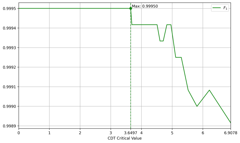
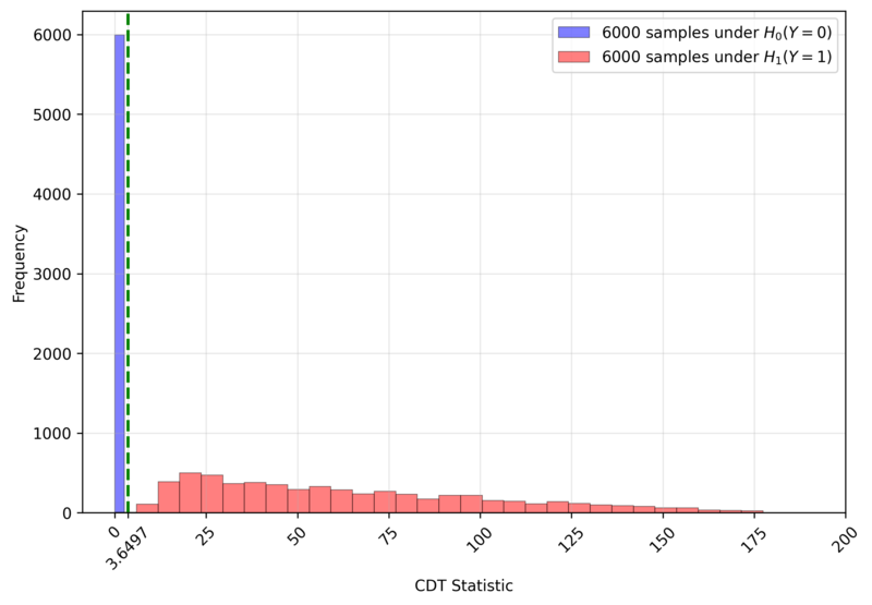
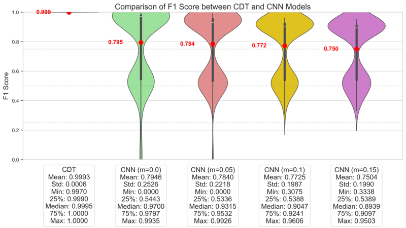
Figure 13 displays the $F_1$-Score distributions for both models over 200 runs. CDT consistently achieves high $F_1$-Scores with low variance, demonstrating stable and high performance. In contrast, the CNN's $F_1$-Score distribution is distinctly bimodal, indicating high variance. This suggests that the CNN's success is highly dependent on the specific dataset composition, undermining its reliability. The lower-performance mode likely corresponds to runs where sufficient training failed. Even when considering only the high-performance mode, the CNN is inferior to CDT in both average performance and stability. Even if the CNN's architecture or learning techniques were improved, its significant computational cost would remain a disadvantage, making CDT a more practical choice.

This outcome stems from the nature of the data. The random location of defective channels means there are no consistent local spatial patterns for a CNN to learn, making DUTMAPs inherently difficult for CNNs to classify. A more reasonable perspective is to view a DUTMAP not as an 'image' with spatial patterns, but as area-wise 'count' data ($|A|, \tilde{x}$). CDT is the direct implementation of this viewpoint.

3.2.Simulation 2: Robustness Analysis

The second simulation evaluates the robustness of CDT by assessing its performance across the entire parameter space of $(d, p_{D^c})$. We generated 100 DUTMAPs for each $(d, p_{D^c}) \in {0, 1, \ldots, 31} \times {3.125\%, 12.5\%, \ldots, 96.875\%}$ and computed the average of the CDT statistic $T(|A|, |A^c|, \tilde{x})$.

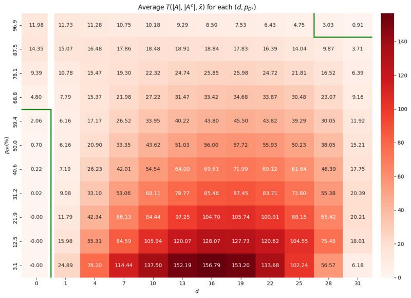
The results are presented as a heatmap in Figure 14. The green line represents the decision boundary where the average CDT statistic equals the critical value of $3.6497$ determined in Section 3.1. Simulation 1. Two areas of vulnerability were identified:

1. False Postive Area: where $d=0$ but $p_{D^c}$ is high (e.g., $\ge 68\%$):
   - In this area the high failure probability leads to $A$ of random failures that are mistaken for the region of defective channels.
2. False Negative Area: where both $d$ and $p_{D^c}$ are extremely high:
   - Here, the signal from the channel defect is obscured by the overwhelming noise from background failures.

Both vulnerability zones correspond to scenarios with extremely low yield. In a real-world manufacturing context, such conditions would likely halt production for root cause analysis and yield improvement, rather than proceeding with mass production. Therefore, these two scenarios are of little practical concern. The results demonstrate that CDT is a robust methodology within the vast majority of the parameter space, which corresponds to almost realistic manufacturing environments.

4. Conclusion

This study proposes Channel Defect Test (CDT), a training-free statistical hypothesis testing method to detect BCIFs on channel-sharing test boards. CDT computes the likelihood ratio between the structural channel-defect hypothesis and the global-random-failure hypothesis using only the observed DUTMAP and the known channel layout. Simulations demonstrate that CDT achieves high detection performance and stability across realistic manufacturing conditions. Vulnerabilities appear only under extreme scenarios with very high background failure rates or many simultaneous defective channels, which are of limited practical concern.

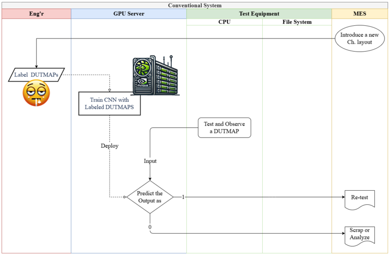
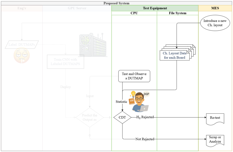
In contrast to CNN-based systems that rely on engineers and a GPU server, as shown in Figure 15, CDT substantially reduces deployment cost and operational complexity. Since the only cost to CDT is the computation of Equation 1, CDT can run in real time on low-end CPUs. This allows it to be embedded as lightweight software in test equipment to detect BCIFs immediately after testing and automatically trigger re-test procedures, as illustrated in Figure 16. This streamlined arrangement is expected to significantly reduce maintenance costs and processing delays. Given the relative lack of prior work on DUTMAP-based BCIF detection, CDT offers a practical, resource-light alternative and a leading approach for accelerating field deployment in this domain.

References

1. Stefan R Vock, OJ Escalona, Colin Turner, and FJ Owens. Challenges for semiconductor test engineering:
A review paper. Journal of Electronic Testing, 28(3):365–374, 2012.

2. Tongwha Kim and Kamran Behdinan. Advances in machine learning and deep learning applications towards
wafer map defect recognition and classification: a review. Journal of Intelligent Manufacturing, 34(8):3215–
3247, 2023.

3. KIM Keunseo, LEE Jaecheol, YANG Minkyu, JANG Jinsic, et al. Method and apparatus with test result
reliability verification, March 13 2025. US Patent App. 18/828,022.

4. Ming-Ju Wu, Jyh-Shing R. Jang, and Jui-Long Chen. Wafer map failure pattern recognition and similarity
ranking for large-scale data sets. IEEE Transactions on Semiconductor Manufacturing, 28(1):1–12, 2015.
doi: 10.1109/TSM.2014.2364237.

5. George Casella and Roger Berger. Statistical inference. Chapman and Hall/CRC, 2024.

6. Yann LeCun, L´eon Bottou, Yoshua Bengio, and Patrick Haffner. Gradient-based learning applied to document
recognition. Proceedings of the IEEE, 86(11):2278–2324, 2002.